Rules of Bingo

Let’s start with the rules of Bingo. Each Bingo card is a 5x5 square. The goal is to cover a complete row, column, or diagonal. Initially, the center (a “free space”) starts covered. The remaining 24 squares each contain a distinct number from 1-75. For the purpose of this post, the free space and diagonals are an annoying complication, so I will assume throughout that there is no free space, and that a win can only come from covering a row or column (not a diagonal).

An important fact is that the numbers on each Bingo card are not totally random: the first column (called the ‘B’ column) always contains 5 random numbers from 1-15; the second (‘I’) column contains 5 numbers from 16-30; the third (‘N’) column contains numbers from 31-45, the fourth (‘G’) contains numbers from 46-60, and the fifth (‘O’) contains numbers from 61-75.

Once every player has their card, the numbers from 1-75 are drawn uniformly at random. When a number is drawn, players cover that number if it appears on their card. When a player has covered a complete row or column, they win and yell “BINGO!”

Method of analysis: many players

The fact that earlier rows have lower numbers is a funny quirk, but why does it matter? In some sense, it doesn’t: if you play bingo alone, the chance that you win by completing a row is exactly the same as the chance that you win by completing a column. But once you have a large number of people playing simultaneously, it turns out that the winner is more likely to complete a row than a column. Why is this?

To start, let’s define some variables. Let \(d\) be the dimension of the Bingo square, and let \(s \ge d\) be the size of the set from which values in each column are drawn (so for real Bingo, \(d = 5\) and \(s = 15\)). Let \(n\) be the number of people playing. Let \(P_R(d,s,n)\) denote the probability that the winning player completes a row, and \(P_C(d,s,n)\) denote the probability that the winning player completes a column. It is possible that the first row and first column are completed simultaneously (by a single player or by different players); let \(P_T(d,s,n)\) denote the probability of such a tie.

The article The Bingo Paradox analyzes the case where the number of players \(n \rightarrow \infty\). You might think that this means that we will always have a winner after the first five numbers are drawn, but this is not correct. This is due to the way Bingo cards are constructed: if the first five balls consist of 3 numbers from the ‘B’ column and 1 number from each of columns ‘N’ and ‘G’, then it is not possible for anyone to have won. Thus, when \(n = \infty\), the game is won as soon as either (i) some column has been drawn for the fifth time, or (ii) all columns have been drawn at least once.

Call a permutation of the numbers 1-75 a ‘column sequence’ if (i) happens before (ii), and a ‘row sequence’ if (ii) happens before (i). (Notice that (i) and (ii) cannot occur simultaneously – that is, as \(n\rightarrow \infty\), there will be no ties.) The authors of the Bingo Paradox article show that when \(d = 5\) and \(s = 15\), row sequences are more than three times as likely as column sequences. Although they do a good job of explaining the calculations, they don’t provide much intuition. Why do rows have an advantage, and how does the probability of a row win depend on \(d\) and \(s\)?

Building Intuition

When trying to develop intuition for this phenomenon, two explanations came immediately to mind. The first was that there are more possible rows than columns. The second was that because there are only \(15\) possible numbers from each column, columns that have already appeared are less likely to be drawn in the future. I discuss each fact below.

Balls in Bins Problem

If we fix \(d\) and take \(s \rightarrow \infty\), the columns from which we draw balls become approximately iid uniform, and this becomes a “balls in bins” problem: imagine the columns as representing different “bins”, and each number drawn is a “ball” that goes into one of these bins.

A row wins as soon as we have at least one ball from each column. This is known as the “coupon collector’s problem”, and it has been well-studied. The expected number of draws required for each of \(d\) columns to turn up is \(d(1 + 1/2 + 1/3 + \cdots + 1/d) \approx d \log(d)\). (When \(s\) is finite, this provides an upper bound on the expected time until each of the \(d\) columns appears, as new columns are always more likely to be drawn than columns that have already appeared.)

Meanwhile, a column wins as soon as some column has appeared \(d\) times. That is, as soon as the bin with the most balls has \(d\) balls. How long do we expect this to take? The number of balls in each bin follows a Binomial distribution with parameters \(m\) and \(1/d\). Thus, it has mean \(m/d\) and variance \(m*(d-1)/d^2 < m/d\). From there, we can apply Chebyshev’s inequality to conclude that if \(m = \alpha*d^2\) for some \(\alpha < 1\), then the probability that a particular column has appeared \(d\) times after \(m\) draws is at most \(\frac{1}{d}\frac{\alpha}{(1-\alpha)^2}\). Applying a union bound across all \(d\) columns gives a probability of a column win of at most \(\frac{\alpha}{(1-\alpha)^2}\).

This bound is fairly loose; tighter bounds are possible with Chernoff bounds, and the distribution of the maximum load after dropping \(m\) balls into \(n\) bins has been studied by the 1998 paper “Balls into Bins: A Simple and Tight Analysis” by Raab and Steger. Rather than going into the details, I want to focus on the high-level point: we need to draw \(\mathcal{O}(d^2)\) numbers before we have a reasonable chance of a column win, and by this time a row win is overwhelmingly likely (as this takes only \(d \log(d)\) draws on average). When \(d\) is large, this will mean that a row win almost always happens before a column win.

I claim also that this conclusion should apply for any \(s\) (so long as \(n = \infty\)) taking \(s \rightarrow \infty\) only decreases the chance of a row win.

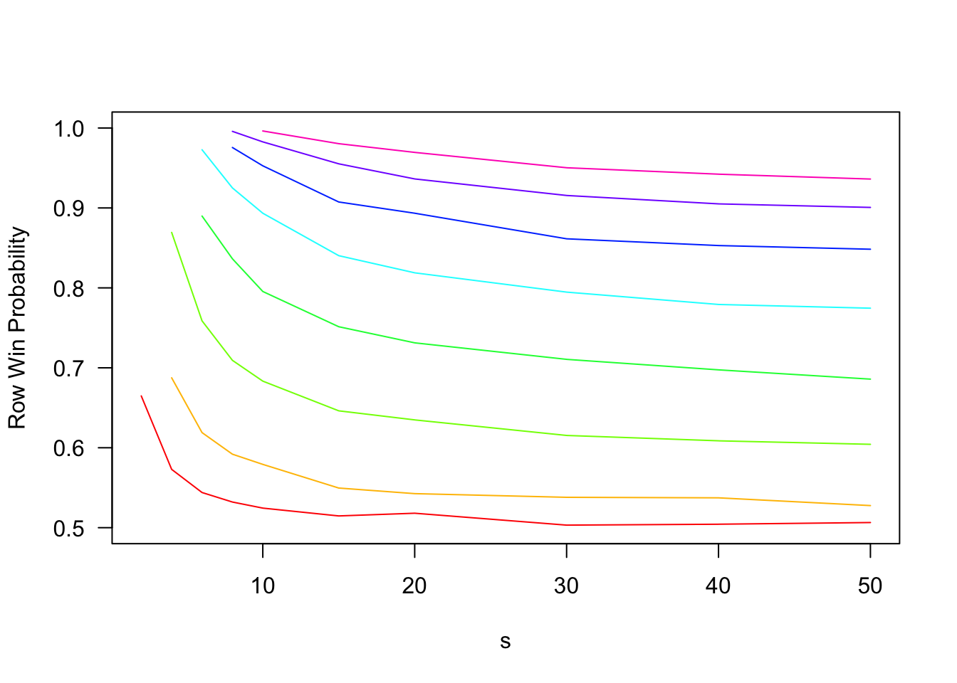
The following code simulates and plots the probability of a row win for various \(d\) and \(s\). The key things to note are (i) increasing \(d\) substantially increases the probability of a row win, and (ii) increasing \(s\) decreases the probability of a row win, but has quickly diminishing marginal returns. Even as \(s \rightarrow \infty\), rows are significantly more likely to win. To take one example, if \(d = 5\), rows win approximately \(94\%\) of the time when \(s = 5\), \(75\%\) of the time when \(s = 15\), and approximately \(67\%\) of the time as \(s \rightarrow \infty\).

first_possible_row_win = function(column_sequence, d){
	columns = unique(column_sequence)
	if(length(columns)>d){ return(NA) } #More columns than there should be
	if(length(columns)<d){ return(Inf) } #No win yet
	if(length(columns)==d){ return(max(match(columns,column_sequence))) } #Last time a new column appears
}

first_possible_column_win = function(column_sequence,d){
	counts = ave(seq_along(column_sequence), column_sequence, FUN = seq_along) #counts[i] returns how many times sequence[i] has appeared so far
	i = which(counts>=d)[1]
	if(is.na(i)){ return(Inf) } #No win yet
	return(i) #Column win after i draws
}


#Generage bingo cards
generate_bingo_cards = function(n_cards,n_row = 5,n_column = 5,available_numbers = c(list(1:15),list(16:30),list(31:45),list(46:60),list(61:75)),free_space = FALSE){
	cards = list()
	for(t in 1:n_cards){
		B = matrix(NA,nrow=n_row,ncol=n_column)
		for(i in 1:n_column){
			B[,i] = sample(available_numbers[[i]],n_row)
		}
		if(free_space){
			B[(n_row+1)/2,(n_column+1)/2] = 0
		}
		cards = append(cards,list(B))
	}
	return(cards)
}

#Combine row sets and column sets from given bingo cards
generate_winning_sets = function(bingo_cards){
	row_sets = c()
	column_sets = c()
	for(B in bingo_cards){
		column_sets = cbind(column_sets,B)
		row_sets = rbind(row_sets,B)
	}
	return(list(row_sets,column_sets))
}

#Given sets of winning rows and columns, as well as an order in which balls are drawn, determine time of first row win and column win
determine_winner = function(row_sets,column_sets,draw_order){
  #Code below assumes that draw_order contains numbers from 1:length(draw_order)
	number_draw_times = match(sort(draw_order),draw_order) 
  
  row_draw_times = matrix(number_draw_times[row_sets],nrow=nrow(row_sets))
	row_win_times = matrix(apply(row_draw_times,1,max))
	
	column_draw_times = matrix(number_draw_times[column_sets],nrow=nrow(column_sets))
	column_win_times = matrix(apply(column_draw_times,2,max))

	#Return time of first row and column winners
	return(c(min(row_win_times),min(column_win_times)))
}

#Do the following n_samples times:
#1. Generate n (d,s)-bingo cards iid 
#2. Simulate a bingo number sequence, determine time of first row win and column win
simulate_bingo = function(d,s,n,n_samples){
	M = matrix(1:(s*d),nrow=s)
	number_sets = split(M,col(M)) #Create list of possible column values
	
	win_times = matrix(NA,nrow=n_samples,ncol=2)
	for(t in 1:n_samples){
		draw_order = sample(unique(unlist(number_sets)))
		column_sequence = 1+floor((draw_order-1)/s) #Assumes number_sets[k] =  ((k-1)*s+1):(k*s)
		win_times[t,1] = first_possible_row_win(column_sequence,d) 
		win_times[t,2] = first_possible_column_win(column_sequence,d) 
		if(n!=Inf) {
		  #Generate set of bingo cards and determine winning sets
		  cards = generate_bingo_cards(n,n_row=d,n_column=d,available_numbers = number_sets) 
		  winning_sets = generate_winning_sets(cards)
		  #Determine time of first row and column win
			win_times[t,] = determine_winner(winning_sets[[1]],winning_sets[[2]],draw_order)
		}
	}
	return(win_times)
}


d = 5 #Dimension of bingo board
s = 15 #Number of possible values in each column
n = Inf #Number of bingo boards to sample
n_samples = 10000 #Number of Bingo simulations to run

outcomes = simulate_bingo(d,s,n,n_samples)
sum(outcomes[,1]<outcomes[,2])/n_samples #Fraction of row wins

## [1] 0.7562

sum(outcomes[,1]>outcomes[,2])/n_samples #Fraction of column wins

## [1] 0.2438

row_win_probability = Vectorize(function(s){
	outcomes = simulate_bingo(d,s,n,n_samples)
	return(sum(outcomes[,1]<outcomes[,2])/n_samples)
})

D = 2:9
colors = rainbow(length(unique(D)))
n = Inf
n_samples = 20000
s = c(2*(1:5),15,20,30,40,50)
plot(NA,xlim=c(min(s),max(s)),ylim=c(1/2,1),las=1,ylab='Row Win Probability',xlab='s')
for(i in 1:length(D)){
	d = D[i]
	lines(s[which(s>=d)],row_win_probability(s[which(s>=d)]),col=colors[i])
}

In this graph, each colored line represents a different choice of \(d\) from \(2\) to \(9\) (\(d = 2\) is the red curve on the bottom, and \(d = 9\) the pink curve at the top). Note that the effect of increasing \(s\) is fairly modest, while increasing \(d\) dramatically increases the probability of a row win.

Simulations for finite \(n\)

All of the above analysis assumed \(n = \infty\). This is very convenient: it allows us to focus only on the columns of drawn balls, and it ensures that there will never be a tie between rows and columns. However, it also requires \(n\) to be very very large! As mentioned above, there are \(s^d\) possible rows, and each card contains only \(d\) of them. Thus, we need at least \(n \ge s^d/d\) players to cover all possibilities (and that is assuming we get to choose the cards). For \(d = 5\) and \(s = 15\), this means over \(150,000\) bingo players!

For smaller \(n\), the row advantage is not so pronounced. For example, the Bingo Paradox article simulated a game with \(n = 1000\), and found that row wins were almost twice as likely as column wins (versus more than 3 times as likely when \(n = \infty\)). When I tried simulating 10000 draws with \(n = 100\), I got 5556 row wins, 4106 column wins, and 338 ties.¹

In fact, if we fix \(n\) and take \(s \rightarrow \infty\), then a fair game is restored!

Claim. Fixing \(d\) and \(n\), \(P_R(d,s,n) - P_C(d,s,n)\) is decreasing in \(s\), and tends to zero as \(s \rightarrow \infty\).

One simple argument to support this claim is that the total number of numbers drawn from each column set is \(d*n\). If \(s\) is extremely large, it is likely that there is no overlap in the numbers that appear on each card. If this happens, there is no longer any structure to the problem: rows and columns will be equally likely to win. However, for this argument to apply, we need \(s\) to be enormous. This is not practical in real-world scenarios, as games of Bingo would take forever with so many numbers to draw!

However, this does show the importance of being precise about the order in which limits are taken: although \(\lim_{s \rightarrow \infty} P_R(d,s,n) - P_C(d,s,n) = 0\) for all \(n\), we have \(\lim_{s \rightarrow \infty} \lim_{n \rightarrow \infty} P_R(d,s,n) - P_C(d,s,n) > 0\).

Closing Thoughts

The Bingo paradox is just one of many examples where probability can be counter-intuitive, even for people like me with a lot of training. When I started thinking about it, my goal was to come up with a way to estimate the row advantage, as a function of \(d, s\), and \(n\), or at least as a function of \(d\) and \(s\) as \(n \rightarrow \infty\).

I haven’t achieved this goal, but I do think I understand the problem better. Intuitively, I expect the following (though I have not proved these statements):

• The row advantage \(P_R(d,s,n) - P_C(d,s,n)\) is always non-negative.
• The row advantage is increasing in \(n\) and \(d\), and decreasing in \(s\).

I especially like the idea of using balls in bins models to lower bound the advantage for \(n = \infty\) and any \(s\). This shows that the unfairness is not primarily caused by \(s\) being too small. When \(n = \infty\), the game becomes increasingly unfair as \(d\) grows, regardless of \(s\). Getting good approximations for finite \(d\), \(s\), and \(n\) remains an interesting problem for future study.