Today, my wife and I dropped my daughter off with grandma, so that we could have a “date morning.” My mom asked what our plans were. We said that we were going to a cafe, order some drinks, and talk about math. And that is exactly what we did. It was great. (I love my wife.)
More specifically, I taught Amanda about linear programming, in a way that I wish I had been taught. I decided to reproduce our conversation in this blog post (extremely silly motivating example and all). For those who have seen linear programming duality before, there are no “new ideas” here. But if duality has always felt a bit like a magical black box, you may find this walkthrough illuminating. And for those who have not seen linear programming: if you have a solid grasp of 8th grade algebra, a pen, a piece of paper, and a little time, this post should be accessible to you!
Introduction
You run a small business that makes and sells things that float. More specifically, you make two products: boats and jetskis. These products don’t emerge out of thin air: they are made from raw materials. Specifically, to make these products you need engines and siding (in reality, a few other things might also be needed, but for our example, these are the only necessary inputs). Each boat requires an engine and three pieces of siding. Meanwhile, a jetski requires two engines, and only one piece of siding. You currently have 17 pieces of siding and 22 engines. You earn \(7\) for each boat and \(5\) for each jetski that you make (if you want, think of this as $7,000 and $5,000). What mix of boats and jetskis should you make to maximize your profit?
Guess and Check
If you really want the full experience, pause here for a couple of minutes, and try to figure out the solution. For example, you could make 4 boats, and 5 jetskis. This would require 17 pieces of siding and 14 engines (leaving you with 8 engines), and would earn 53. Alternatively, you could make 2 boats and 10 jetskis, which requires 16 pieces of siding and 22 engines (leaving you with 1 extra piece of siding), and earns 64. Is a better plan out there? How could we know we have the best plan?
Algebra
We can organize our work as follows. Let \(B\) be the number of boats that we decide to produce, and \(J\) the number of jetskis. Then we must have \[\begin{equation} B + 2J \le 22 \label{eq:engine} \end{equation}\] \[\begin{equation} 3B + J \le 17 \label{eq:siding} \end{equation}\] This is because \(B + 2J\) gives the number of engines we need, and \(3B + J\) gives the number of pieces of siding that we need. Of course, we also must have \[\begin{equation} B \ge 0, J \ge 0 \label{eq:bjpositive} \end{equation}\] Our revenue (in thousands of dollars) is \(7B + 5J\). So our goal is to choose \(B\) and \(J\) to maximize this revenue, subject to \(\eqref{eq:engine}\) \(\eqref{eq:siding}\), and \(\eqref{eq:bjpositive}\).
Geometry
Let’s plot the feasible region defined by \(\eqref{eq:engine}\) \(\eqref{eq:siding}\), and \(\eqref{eq:bjpositive}\)
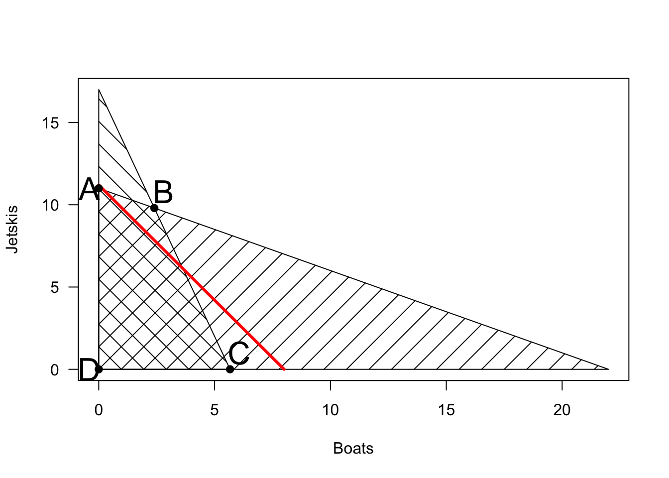
The space of possible production plans is the cross-hatched region, which does not depend on the sales prices of boats and jetskis. To choose the best production plan, we need to consider these prices. We can plot “indifference curves” (sets of production plans that produce identical revenue). For example, the line in red shows all production plans that yield exactly 56 in revenue (it is the line \(7B + 5J = 56\)). As we set higher and higher revenue targets, the line moves up and to the right, until eventually, there are no feasible production plans that achieve this revenue.
Visually, it is clear that the last point of contact with the feasible region will be the point marked ‘B’. This is the intersection of the lines \(B + 2J = 22\) and \(3B + J = 17\), which is \((B,J) = (2.4,9.8)\). So it says to make \(2.4\) boats and \(9.8\) jetskis, which results in a profit of \(65.8\). (Of course, in reality, a fractional production plan doesn’t make much sense – what does it mean to make 9.8 jetskis? It turns out that if we constrain \(B\) and \(J\) to be integers, the problem becomes an integer programming problem, which is much harder. If the fractional numbers bother you, imagine that we have 220 engines and 170 pieces of siding, in which case our solution would be to make 24 boats and 98 jetskis).
Note that point \(B\) would remain the optimal solution for many sales prices for boats and jetskis. In general, for any prices, one of the extreme points in black will always be optimal. The prices determine the slope of the red “indifference lines.” If jetskis are much more valuable than boats, the line will be more horizontal (and we may choose point \(A\)). If boats are much more valuable than jetskis, the line will be vertical, and we may choose point \(C\). For many prices, we will end up choosing \(B\). (And if both prices are negative, we would choose point \(D\)).
Duality: Obtaining an Upper Bound
If we had more than 2 variables and 2 equations, solving for an optimal plan seems hard. But coming up with a feasible plan and calculating its associated profit is pretty easy. For example, suppose that we planned to make 2 boats and 10 jetskis. It’s easy to see that this is feasible, and that its associated profit is \(2 \times 7 + 10 \times 5 = 64\).
We wish to know how far this plan is from optimal. Here is an argument to show that NO feasible plan can earn more than 78.
Let \(B\) and \(J\) be a feasible plan. From \(\eqref{eq:engine}\) they must satisfy \(B + 2J \le 22\), and therefore \(2B + 4J \le 44\). From \(\eqref{eq:siding}\), they must satisfy \(3B + J \le 17\), and therefore \(6B + 2J \le 34\). Adding these two inequalities together, we get \[\begin{equation} 8B\tag{1}8. (#eq:bound) \end{equation}\] In other words, even if we sold boats for 8 and jetskis for 6, we could not make more than 78. In reality, we sell boats for 7 and jetskis for 5, so of course our optimal profit must be even less.
Pause here to internalize this argument. Do you follow it? Can you adapt it to come up with a better upper bound?
There are many ways to do this. For example, we could triple \(\eqref{eq:siding}\) and ad it to \(\eqref{eq:engine}\) to get \(10 B + 5 J \le 73\). Thus, even if we could sell boats for 10 and jetskis for 5, we could not earn more than 73.
On the other hand, we could take the equation we discovered (1), and multiply the whole thing by \(7/8\) to get \(7B + 5.25 J \le 69.75\).
A General Approach To Finding Upper Bounds
How can we come up equations to formalize and generalize this approach to finding upper bounds? In general, all of the bounds above took the form of multiplying our engine constraint \(\eqref{eq:engine}\) by some number \(U\), and our siding constraint \(\eqref{eq:siding}\) by another number \(V\) and adding them together. We can’t just choose any \(U\) and \(V\) we want: we need the eventual coefficient on \(B\) to be at least \(7\) (our revenue from selling a boat), and our eventual coefficient on \(J\) to be at least 5 (our revenue from selling a jetski).
In other words, we must have \[\begin{equation} U + 3 V \ge 7 \label{eq:boat} \end{equation}\] \[\begin{equation} 2U + V \ge 5 \label{eq:jetski} \end{equation}\] The bound we end up with is \(22U + 17V\).
There is one more constraint on \(U\) and \(V\) that we have left off. We need \[\begin{equation} U \ge 0, V \ge 0 \label{eq:uvpositive} \end{equation}\] Why? If \(U < 0\), then when we multiply it by \(\eqref{eq:engine}\), the inequality would flip signs.1
So our goal is to choose multipliers \(U\) and \(V\) to get the best possible upper bound. In other words, we wish to minimize \(22U + 17V\), subject to \(\eqref{eq:boat}\), \(\eqref{eq:jetski}\), \(\eqref{eq:uvpositive}\). Note that this is itself a linear program (called the dual of the original linear program)!
Interpreting the Dual
Before moving on, let’s see if we can interpret the quantities \(U\) and \(V\). In our original linear program, \(B\) and \(J\) were easily interpretable as the number of boats and jetskis we should make. What do \(U\) and \(V\) represent?
Well, there are some hints. First of all, \(U\) is associated with the engine constraint, and \(V\) with the siding constraint. In general, we should have one multiplier variable for each raw material (constraint) in the original problem. Second, we know that the expression \(22U + 17V\) (our upper bound) should have units of dollars. Since 22 represents the number of engines we have on hand, and 17 the number of pieces of siding, it must be that \(U\) has units of dollars per engine, and \(V\) of dollars per piece of siding.
The usual interpretation that is given is, suppose that a businessperson wishes to buy our business from us. They offer us \(U\) for each engine, and \(V\) for each piece of siding that we have on hand. Which choices of \(U\) and \(V\) are high enough that we accept their offer? Certainly, it must be the case that \(U + 3V \ge 7\) (that is, \(\eqref{eq:boat}\) holds), or else we could simply do better by turning our materials into boats. Similarly, we must have that \(2U + v \ge 5\), or we would turn the businessperson down and make jetskis. The dual linear program is trying to figure out the lowest prices that the businessperson can offer which would cause us to accept.
Now that we have a clearer interpretation of the dual, let’s go back to its usefulness. In fact, let’s put the original problem (called the “primal”) side by side with the dual.
\[\begin{align*} (Primal) \hspace{.4 in} \max & \hspace{.2 in} 7B + 5J \\ s.t. & \hspace{.2 in} B + 2J \le 22 \\ & \hspace{.2 in} 3B + J \le 17 \\ & \hspace{.2 in} B, J \ge 0 \end{align*}\] \[\begin{align*} (Dual) \hspace{.4 in} \min & \hspace{.2 in} 22U+17V \\ s.t. &\hspace{.2 in} U + 3V \ge 7 \\ & \hspace{.2 in}2U + V \ge 5 \\ &\hspace{.2 in} U, V \ge 0 \end{align*}\]
Algebraically, these problems don’t seem especially related. I mean, clearly they use some of the same numbers, but the actual variables are different, and represent very different things.
And yet, what we have just argued is that any feasible solution of the dual gives us an upper bound on the profit we can earn (i.e. the value of the primal). So for example, when we took \(U = 1, V = 3\), we got \(22U + 17V = 73\), indicating that no plan can earn more than 73. It is also true that any feasible solution to the primal gives a lower bound for the value of the dual. In other words, the fact that we came up with a production plan (2 boats and 10 jetskis) that earns us a profit of 64 means that the businessperson needs to offer us at least 64 in order to get us to sell. This magical relationship between the primal and dual is called “weak duality.”
Weak duality can be very useful for obtaining bounds, but what if we want the exact optimal solution? In this problem, we can guess that the best bound we could hope for with this method will be one where the coefficient on \(B\) is exactly \(7\), and the coefficient on \(J\) will be exactly \(5\). Solving \(U + 3V = 7\) and \(2U + V = 5\) yields \(U = 1.6, V = 1.8\). When we choose these values, we get \(22 U + 17V = 65.8\).
Notice that the value of this bound exactly matches the value we got when we chose \(B = 2.4, J = 9.8\) in the original problem. In other words, we now have a plan that earns a profit of 65.8 (\(B = 2.4, J = 9.8\)), as well as a proof that no plan can earn a higher profit (\(U = 1.6, V = 1.8\)). So we have found the optimal solution! It turns out that in general, a primal and its dual will have the same objective value (there is no gap between them). Thus, it is always possible to come up with this type of proof of optimality. This is called “strong duality.”
Notice that the optimal dual variables \(U = 1.6, V = 1.8\) also tell us whether it is worthwhile to buy additional siding and/or engines. In essence, \(U\) is saying that each additional engine could increase our total profit by \(1.6\), while \(V\) says that each additional piece of siding could increase our total profit by \(1.8\). This is pretty useful information!
Background Information on Linear Programming
The problem above is a special case of what is called a linear programming problem. The key features of linear programming are: 1. The constraints that determine the feasible region are linear. 2. The objective is linear.
In other words, nowhere in the constraints do we see \(B^2\) \(\sqrt{J}\), \(B/J\), \(B \times J\), \(e^{-J}\), or any other similar terms. Linear constraints imply that the feasible region will always have a finite set of extreme points, defined by intersections of linear equations. A linear objective implies that our red “indifference curves” will always be linear (not curved), and that therefore one of the extreme points of the feasible region will end up being optimal.
Of course, when there are more than \(2\) variables and \(2\) equations, drawing pictures and solving the problem by hand gets tricky. The most well-known algorithm for solving these problems in general is called the simplex method. This method starts at one extreme point, and then walks to nearby extreme points until it has found the best one. At each step, the direction of the walk is determined by the goal of increasing the objective value.
While the simplex method always finds the optimal solution, a natural question is, how fast is it? The number of extreme points that define the feasible set can grow exponentially in the number of variables and equations, so if the simplex method has to visit all of these points, it will be very slow. But perhaps the method always takes a direct path to the optimal solution, which only passes through a small number of extreme points?
For a period after the simplex method was discovered, a key open question was weather it always ran “quickly” (in polynomial time). These days, we know that it does not: on some worst-case examples, it visits a “large” (exponential) number of extreme points before finding the optimal solution. Is this a failing of the simplex method, or a sign that linear programming problems are inherently hard?
It turns out that it is possible to solve any linear programming problem in polynomial time. The first algorithms shown to do this are “interior point” algorithms. Rather than walking along the outside edges of the feasible set (as the simplex algorithm does), these algorithms start from a point solidly within the feasible set, and use the objective function to guide an exploration towards an optimal extreme point. Although these methods are faster in the worst case than the simplex method, they tend to be slower on most instances.
Note that if our engine equation had to hold with equality, then allowing \(U\) to be negative would cause no problems. This explains the “rule” I was taught to memorize, which is that equality constraints in the primal result in unconstrained dual variables. But I feel so much better actually understanding where that rule comes from, rather than just accepting it as an article of faith.↩︎