The final unit of my operations course is on inventory management. Among other topics, we study the classic “Newsvendor” model.1 In my first year teaching at Columbia, I came up with a neat visualization of this model. The goal of this post is to share my visualization – hopefully you will agree that it’s helpful!
The Newsvendor Model
You are planning to sell a product – let’s say a new board game that you have developed. You pay a manufacturer to print your game. There are high setup costs, so you are only planning to do a single print run. The problem is, you don’t know how popular your game will be! Thus, you must make an informed guess when deciding a production quantity. Order too many games, and you’ll lose money. Order too few, and you’ll miss out on potential sales!
More formally, in the first period, you face must decide on a production quantity \(q\), and incur a marginal cost of \(c\) for each game produced. Then, demand \(D\) is realized. Your total sales are \(\min(D,q)\), and all sales occur at price \(p\). You do not know demand \(D\) in advance, but capture your uncertainty by assuming that it follows a distribution with cdf \(F\). What production quantity \(q\) maximizes your expected profit?
Several Solutions
The most obvious approach to solve this problem is to calculate expected profit for each order quantity, and then choose the order quantity for which this profit is largest. Although valid, this approach is cumbersome and unilluminating.
Instead of calculating total profit, it is more helpful to think about marginal profit from producing one more copy.2 Presumably, you are certain to sell the first copy you produce – at the very least, your parents will take pity on you and buy it! However, if you are already planning to make \(10,0000\) copies, then printing additional copies may not be a great idea: they will help you only if demand exceeds \(10,000\). More precisely, if I move from producing \(q\) copies to producing \(q+1\), I will pick up an extra sale whenever demand is greater than \(q\), but will incur additional production costs, resulting in regret when demand is less than or equal to \(q\). Thus, the marginal benefit from the \((q+1)^{st}\) copy produced is \[MB(q+1) = P(D > q) p - c = (1 - F(q))p-c.\] This is positive so long as \(F(q) \leq 1 - c/p\), so I want to increase my order quantity \(q\) until my probability of having excess inventory (that is, \(P(D < q)\)) is roughly \(1 - c/p\). The quantity \(1 - c/p\) gets a special name: the “critical ratio.” If you think the chance of being stuck with an extra copy is higher than the critical ratio, then you’re better not producing that copy at all. Note that in this problem, the critical ratio is equal to your profit margin: for very profitable games, you have a high tolerance for excess inventory and low willingness to lose out on sales, so you will produce a large quantity.3
One quick aside. In this scenario, we assume that excess copies are useless, and whenever you have a shortage, you lose the sale. In many business situations, excess inventory will have some salvage value, and you can place backorders if demand exceeds your supply. These possibilities affect the calculations above: in particular, we can still calculate a critical ratio, but it may no longer equal the profit margin. To address this, in general we say that there is some underage cost \(c_u\), representing the regret you experience each time you are short one item, and an overage cost \(c_o\) that you experience for each item that you produce beyond demand. In the example above, the underage cost is the cost of a lost sale \(p - c\) and the overage cost is the production cost \(c\). Once you know the overage and underage costs, the marginal benefit analysis above tells us that we should continue producing copies until our probability of excess inventory equals \(c_u/(c_u+c_o)\), which is the general formula for the critical ratio.
A Visual Approach
Suppose that we produce \(q\) copies. For each \(n \in \{1, \ldots, q\}\), the probability that we sell our \((n+1)^{st}\) copy is \(1 - F(n)\). By linearity of expectation, our total expected sales can be calculated by adding up the sales probabilities of individual items: \[S(q) = \mathbb{E}[\min(D,q)] = \sum_{n = 0}^{q-1} (1 - F(n)).\]
Let’s “see” this visually. Start by plotting the cdf \(F\). Then draw a vertical line at the proposed production quantity \(q\). The equation above implies that our total expected sales \(S(q)\) is the area of the region to the left of our order quantity and above \(F\). In Figure 1, this region is shaded in blue. Once we know our expected sales, we can calculate two other quantities of interest. First, expected excess inventory is \(q - S(q)\), which is equal to the area of the red region. Second, expected lost sales (from lack of inventory) is equal to \(\mathbb{E}[D] - S(q)\), which is equal to the area of the orange region.
Now, we can see the consequences of changing our production quantity: as we move the vertical line to the right, sales increase (lost sales decrease), but so does expected excess inventory! We want to choose our order quantity to strike an appropriate balance: that is, to minimize a weighted sum of the red and orange regions.
This is where the economics of the situation come in. The red and orange regions represent excess inventory and lost sales in quantities of games. We want to translate these to dollars. The critical ratio tells us how costly “overage” is relative to “underage.” More specifically, it tells us how often we should have excess inventory when ordering optimally. We can plot the critical ratio as a horizontal line. This line intersects the demand distribution \(F\) at the optimal order quantity.
plotnews = function(cr,F,qMin = 0, qMax,q){
  plot(F,xlim = c(qMin,qMax), ylim=c(0,1),ylab='P(Excess Inventory)',yaxs='i',xaxs='i',xlab='Order Quantity',las=1) #Plot Demand Distribution
  x = c(qMin:qMax)
  y = F(x)
  polygon(c(x[1:q],x[q],0),c(y[1:q],1,1),col='light blue') #Expected Sales
  polygon(c(x[1:q],x[q],0),c(y[1:q],0,0),col='red') #Expected Excess Inventory
  polygon(c(x[q:qMax],x[q],x[q]),c(y[q:qMax],1,1),col='orange') #Expected Lost Sales
  abline(h=cr) #Plot Critical Ratio
}

cr = 0.6
mean = 100
sd = 30
qStar = ceiling(qnorm(cr,mean,sd))
qMax = mean+3*sd
F = function(x){return(pnorm(x,mean,sd))}

plotnews(cr,F,qMin = 0,qMax,qStar)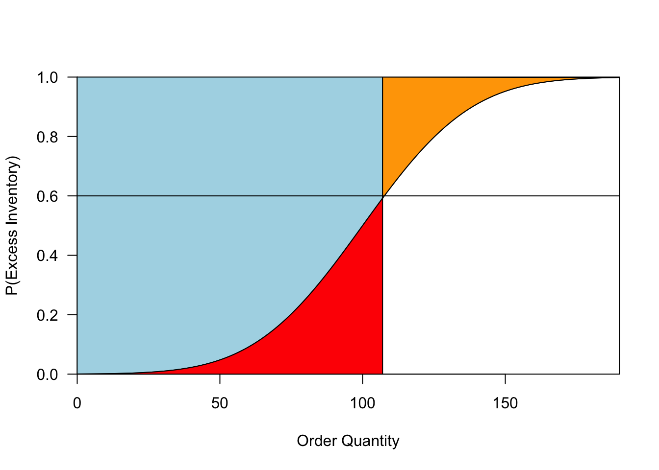
Figure 1: A visualization of the classical newsvendor problem. The curve represents the CDF of the demand distribution. The vertical line gives our order quantity. The blue region represents expected sales, and the red and orange regions represent expected overage and underage, respectively. The horizontal line shows our critical ratio: the optimal order quantity is where this line intersects the demand distribution.
To me, the resulting picture is beautiful. It captures so much about the problem! We know that we’re trying to adjust the production quantity (vertical line) to balance overage (red) and underage (yellow). To determine an optimal order quantity, we need both a demand forecast (\(F\)) and an understanding of the relative costs of overage and underage (the critical ratio). Each of these is represented by a single curve in Figure 1.
Several insights arise.
No matter what demand distribution you draw, you should order so that our probability of excess inventory is equal to the critical ratio.
As the critical ratio increases, so does our optimal production quantity, as shown in Figure 2. When you have a lot of certainty about demand, the distribution \(F\) will rise very steeply. In these cases, changes to the critical ratio do not have a large effect on our production quantity: you roughly produce to match demand. Meanwhile, when demand is very uncertain, the distribution \(F\) will be flatter, and the critical ratio will greatly influence our order.
As you become more certain about demand, \(F\) becomes steeper and both the red and orange regions shrink, as shown in Figure 3. Thus, increased certainty does not change our chance of having overage or underage (see the first insight), but it does decrease the expected amount by which you err. Note also that increased certainty could either increase or decrease your optimal order. Your order will decrease when your critical ratio is high and you were previously hedging by over-ordering (as shown in 3); it will increase when your critical ratio is low.
You don’t need perfect demand information to make reasonable ordering decisions. For example, you can assess whether our current policy systematically over-produces or under-produces using only the critical ratio and knowledge of how frequently you sell out. In addition, if our critical ratio is bounded away from 0 or 1, then you don’t need to account for very rare events that dramatically shift demand.4
plotnews(cr,F,qMin = 0,qMax,qStar)

crNew = 0.8
qNew = ceiling(qnorm(crNew,mean,sd))
abline(h=crNew)
arrows(qStar-1,cr,qStar-1,crNew,lwd=2) #Increase in CR
arrows(qStar-1,crNew,qNew,crNew,lwd=2)

text(85,(cr+2*crNew)/3,"Increased")
text(85,(2*cr+crNew)/3,"Critical Ratio")
text(122,0.93,"Increased")
text(122,.87,"Order")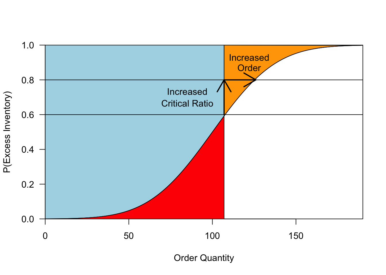
Figure 2: As the critical ratio increases, so does the optimal order quantity. The rate of increase is largest when demand is very uncertain.
cr = 0.8
plotnews(cr,F,qMin=0,qMax, q =  ceiling(qnorm(cr,mean,sd)))

sd = 15
plotnews(cr,F,qMin=0,qMax, q =  ceiling(qnorm(cr,mean,sd)))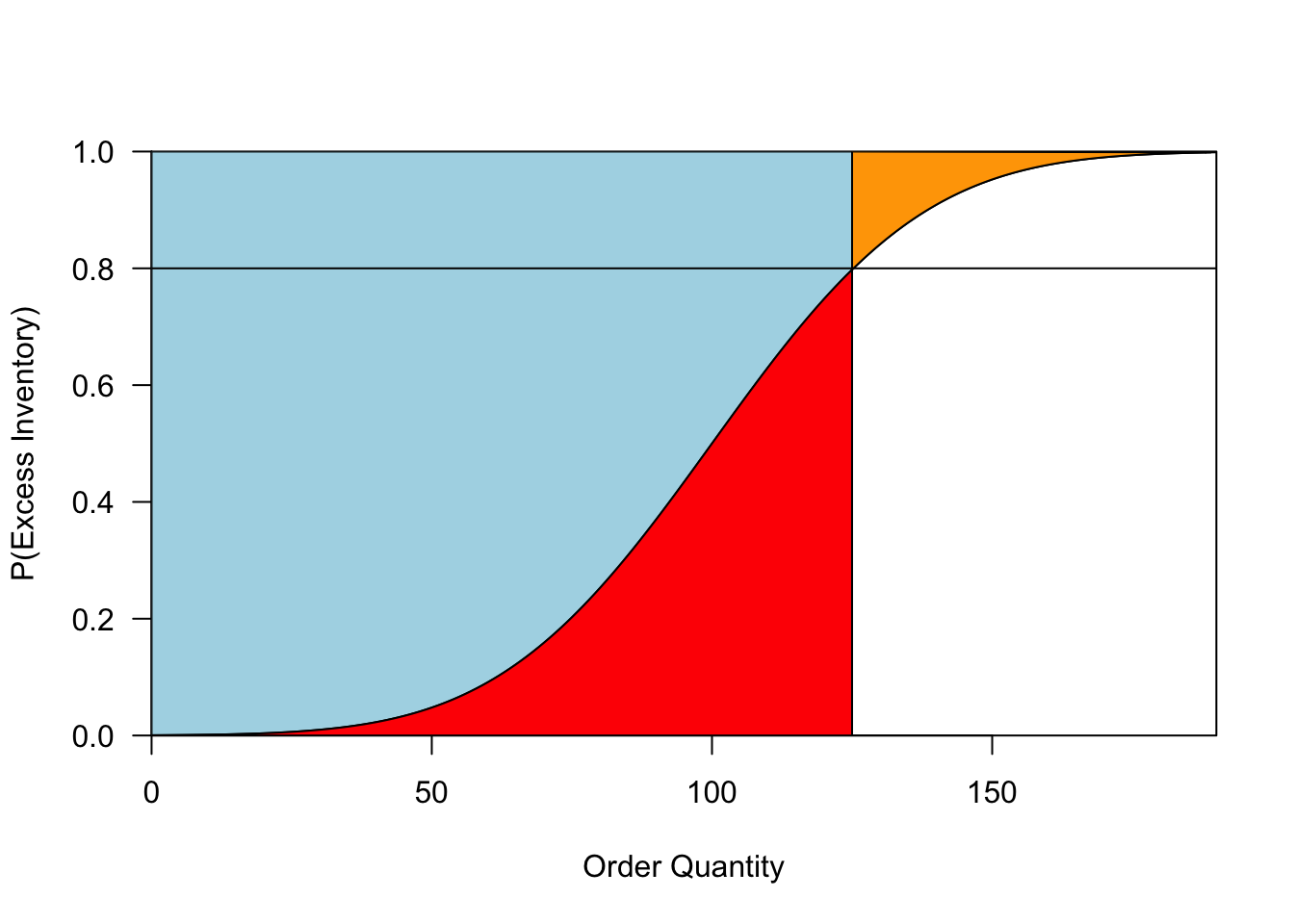
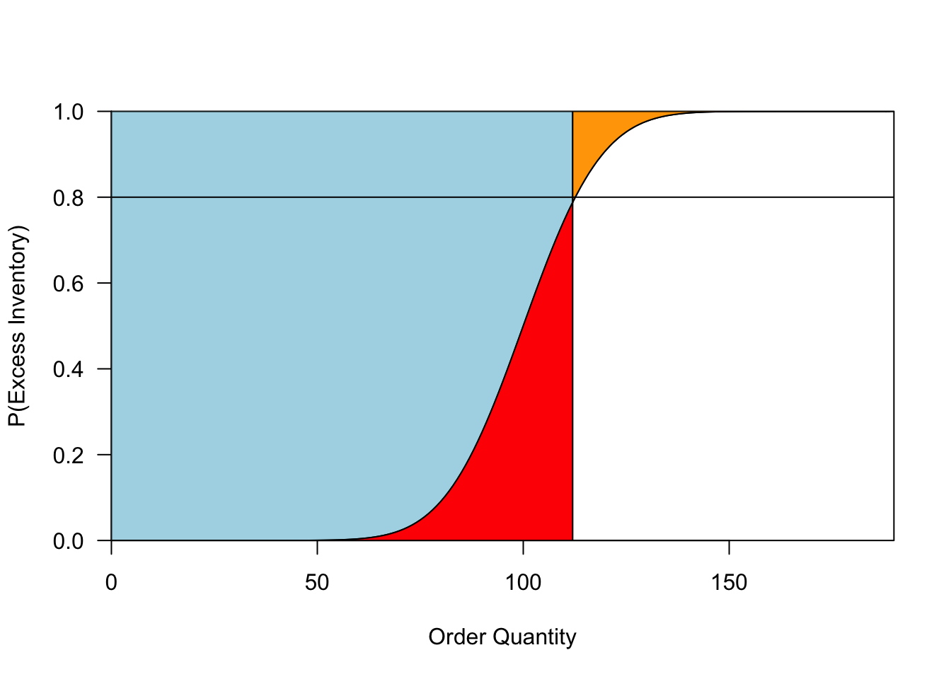
Figure 3: Outcomes when demand is uncertain (left) and more certain (right). When ordering optimally, the probability of having some overage is the same in both cases, but the expected overage and underage (in red and orange, respectively) is much lower when demand is more certain.
This model forms the backbone for many papers in operations. See this previous blog post for one example.↩
For those of you who worry about these things, our objective function is quasi-concave, so first order methods will identify the optimal solution.↩
Note that this is the marginal profit margin, not the average profit margin. That is, the cost \(c\) should not incorporate fixed costs of production.↩
To relate this topic to current events, this helps to explain why companies don’t proactively produce and store vaccines that will only be needed in rare circumstances. For more on vaccine production, see this Planet Money episode.↩