Prologue: Running in Graduate School
The motivation for this post comes from my time in graduate school. A popular run on the Stanford campus is Campus Drive Loop. There are sidewalks on either side of the road, giving the runner a choice of which to take. On days when I felt low-energy, I would sometimes take the inside sidewalk, figuring that this would shorten my run. But by how much?
If the loop were a perfect circle, the answer would be easy – my savings would be \(2 \pi\) times the width of the road, implying a shorter route by something like 300 ft. But as shown in Figure 1, the loop is far from circular, and is not even convex. I wondered, is 300 feet still a reasonable answer, or is it possible that the savings could be much more or much less?
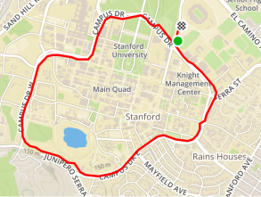
Figure 1: Campus Drive Loop at Stanford University.
After drawing a few simple shapes (mostly compositions of straight lines and partial circles), I became convinced that in fact, the answer was \(2\pi\) times the width of the road, regardless of its shape. But I felt I lacked the tools to tackle the problem formally. This is where my friend Jake Levinson comes in. I posed this question to him while on Safari in Tanzania, and he promptly tackled it with gusto (see Figure 2). He managed to show that for any reasonable running loop, my intuition was correct. However, he also found some interesting exceptions!
At this point, I’ll let Jake take over – the rest of this post is all his.
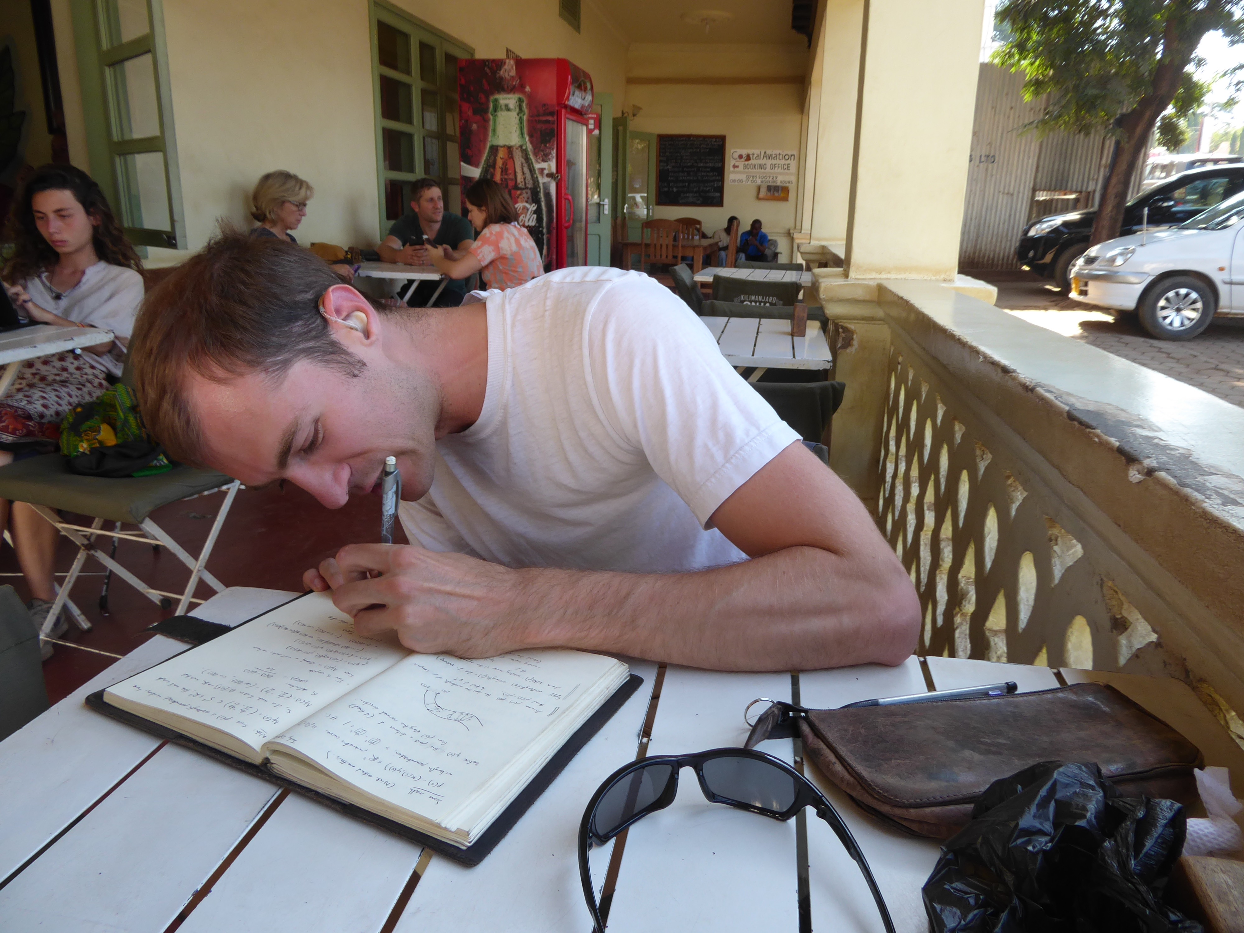

Figure 2: Left: Jake sketching ideas in a cafe in Moshi. Right: how we spent the rest of our time.
Introduction
Two friends are out running together along a winding path, traveling in parallel and at a fixed distance from one another:
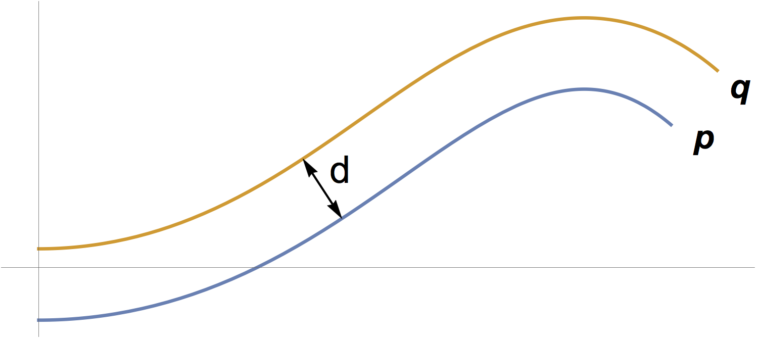
A natural question is, how much longer is the ‘outer path’ than the ‘inner’ path? This question is particularly interesting in the case where both paths are closed loops, so the outer path traces out a ribbon or bounding envelope around the inner path. We’ll show a surprising fact: in most cases, the precise shape of the path doesn’t matter: the difference in lengths is an integer multiple of \(2\pi d\).
Setup
Let \({\bf p}(t)\) and \({\bf q}(t)\) be the two paths in \(\mathbb{R}^2\). So, for some constant \(d > 0\) and all \(t\), \[\begin{equation} \label{eqn:core_assumption} ||{\bf q}(t)-{\bf p}(t)|| = d, \quad \text{and} \quad {\bf q}'(t) \propto {\bf p}'(t). \end{equation}\] We will assume both paths are differentiable closed loops, and set \(t \in [0, 1]\), so \[\begin{align*} {\bf p}(0) = {\bf p}(1), \qquad {\bf q}(0) = {\bf q}(1), \\ {\bf p}'(0) = {\bf p}'(1), \qquad {\bf q}'(0) = {\bf q}'(1). \end{align*}\]Differentiating condition \(\eqref{eqn:core_assumption}\) leads to two possibilities for \({\bf p}(t)\) and \({\bf q}(t)\):
- We have \({\bf q}'(t) = {\bf p}'(t)\), so that \({\bf q}\) is just a translate of \({\bf p}\), or
- We have \({\bf q}(t)-{\bf p}(t) \propto {\bf n_p}(t)\), the normal vector to \({\bf p}(t)\) that is, \({\bf q}\) ‘swerves’ around \({\bf p}(t)\), as illustrated above. (Equivalently, \({\bf p}(t) - {\bf q}(t) \perp {\bf p}'(t).\))
A given pair of paths may switch between cases (i) and (ii) for different values of \(t\), but condition (ii) captures the behavior we want, so we will assume (ii) holds for all values of \(t\). (See Figure 3.)
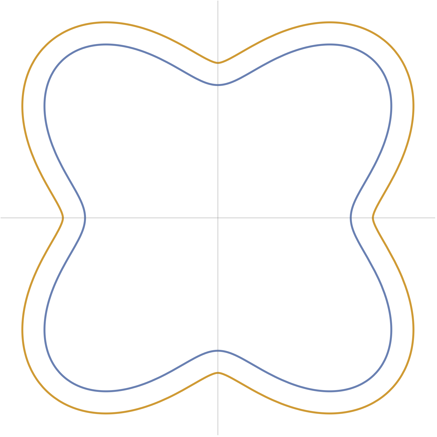
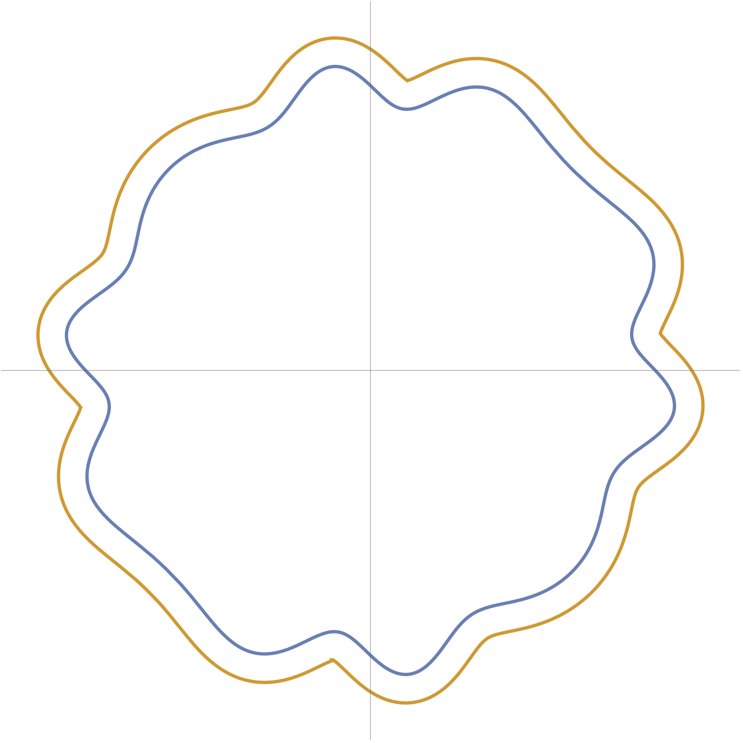
Figure 3: Fixed-distance parallel paths.
With this in mind, the question is: what are the arclengths of \({\bf p}\) and \({\bf q}\)? If the two paths trace out concentric circles (or certain other toy paths, such as rounded squares) it is easy to see that the arclengths differ by exactly \(2\pi d\). One might expect, however, that in general the difference in arclengths may depend on the particular shapes of the paths.
Our main goal is to examine the following surprising fact:
Theorem 1 Suppose \({\bf q}'(t)\) is always a positive multiple of \({\bf p}'(t)\). Then \[arclength({\bf q}) - arclength({\bf p}) = k \cdot 2\pi d\] for some integer \(k \in \mathbb{Z}\). If \({\bf p}\) is a simple closed curve, traced once as \(0 \leq t \leq 1\), then \(k=1\).
We’ll also see a couple of examples of why the ‘positive multiple’ requirement is necessary, and what kinds of exceptional curves you can get otherwise.
Controls
We proceed as follows. Since the path is a smooth curve, \({\bf p}\) is differentiable and \({\bf p}'\) never vanishes. So, without loss of generality (rescaling \(t\) and \(\mathbb{R}^2\) if necessary), we assume \({\bf p}(t)\) is arclength parametrized: \(||{\bf p}'(t)|| = 1\) for all \(t\). Effectively, we assume one of our two ‘runners’ runs at a constant speed along the path, while the other runner speeds up or slows down as necessary to keep pace.
Now, since \({\bf p}'(t)\) is always a unit vector, there exists a differentiable function \(\theta : [0,1] \to \mathbb{R}\) such that \[{\bf p}'(t) = \big(\cos \theta(t),\ \sin \theta(t)\ \big).\] The angle \(\theta\) is just the angle in which the path \({\bf p}(t)\) points – the compass direction the runner is facing at time \(t\). We will see that the important quantity is \(\theta'(t)\), which tells us how fast the runner is turning.
(A similar mathematical setup occurs in other contexts in control theory. It can be helpful to think of \({\bf p}(t)\) as a scooter or motorboat, traveling at constant unit speed, but which is controlled by a driver. The quantity \(\theta(t)\) is the direction the vehicle is facing at time \(t\), while \(\theta'(t)\) is the angle at which the steering wheel is being held.)
Now the arclength of \({\bf p}\) is, by our normalized setup, \[\mathrm{arclength}_{[0,1]}({\bf p}) = \int_0^1 ||{\bf p}'(t)||dt = \int_0^1 1\ dt = 1.\]
We now describe \({\bf q}\). We know that \({\bf q}(t) - {\bf p}(t)\) is always a normal vector to \({\bf p}\) of length \(d\), so we may write \[{\bf q}(t) - {\bf p}(t) = \pm d \cdot {\bf n_p}(t) =\pm d \cdot \big( {-}\sin \theta(t), \cos \theta(t) \big). \] (We have chosen \({\bf n_p}(t)\) counterclockwise to \({\bf p}'\), i.e. \(\{{\bf p}', {\bf n_p}\}\) is positively oriented.) The choice of sign says whether \({\bf q}(t)\) is ‘to the left or right’ of \({\bf p}(t)\). We choose \(-\), so: \[\begin{equation} \label{eqn:q from p} {\bf q}(t) = {\bf p}(t) - d \cdot \big( {-}\sin \theta(t), \cos \theta(t) \big). \end{equation}\]Note that \(\theta', d > 0\) means \({\bf p}'\) turns counterclockwise with \({\bf q}\) to its right.
A motivational computation
We now examine the arclength of \({\bf q}\) and see why usually it is exactly \(2\pi d\) longer than that of \({\bf p}\). We have
\[\begin{align*} \mathrm{arclength}_{[0,1]}({\bf q}) = \int_0^1 ||{\bf q}'(t)|| dt. \end{align*}\] From Equation \(\eqref{eqn:q from p}\), \[\begin{align*} {\bf q}'(t) &= {\bf p}'(t) - d \theta'(t) \cdot \big( {-}\cos \theta(t), \sin \theta(t) \big) \\ &= {\bf p}'(t) + d \theta'(t) \cdot {\bf p}'(t) \\ &= (1+d \theta'(t)) \cdot {\bf p}'(t). \end{align*}\]Since \({\bf p}'(t)\) is a unit vector, \(||{\bf q}'(t)|| = |1+d\theta'(t)|\).
Suppose this quantity is always positive: \[\theta'(t) \geq -\tfrac{1}{d}.\] We will examine this assumption later and see that it has an elegant geometric significance. For now, we just observe that it then follows \[\begin{align*} \mathrm{arclength}_{[0,1]}({\bf q}) &= \int_0^1 ||{\bf q}'(t)|| dt \\ &= \int_0^1 (1+d\theta'(t)) dt \\ &= 1 + d\big( \theta(1) - \theta(0) \big) \\ &= \mathrm{arclength}_{[0,1]}({\bf p}) + d\big( \theta(1) - \theta(0) \big). \end{align*}\]Since \({\bf p}\) is a differentiable closed curve, \({\bf p}'(0) = {\bf p}'(1)\), and so \(\theta(1) - \theta(0)\) is a multiple of \(2\pi\). This multiple is called the winding number of \({\bf p}'\), counting how many times the direction vector \({\bf p}'\) twists all the way around as \(t\) ranges from \(0\) to \(1\).
For many curves encountered in practice, such as running paths – in particular if \({\bf p}\) is a simple closed curve, i.e. does not cross itself – the winding number is \(1\). In other words, \({\bf p}\) turns all the way around once as it circles back on itself. This is self-evident in each of the curves depicted in Figure 3$, so the arclength difference is \(2\pi d\) in those cases. This completes Theorem 1! For other sorts of paths, such as self-crossing spirals, \({\bf p}\) may twist around numerous times (see Figure 4), and the arclengths will differ by larger multiples of \(2\pi d\).
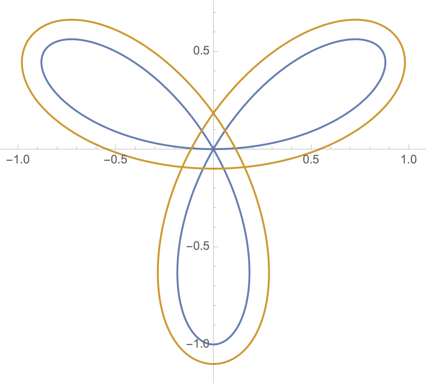
Figure 4: A spiraling, self-crossing curve and its parallel counterpart. Tracing along the inner curve \({\bf p}\), observe that the tangent vector \({\bf p}'\) twists around twice as we traverse the curve (note it is horizontal at \((0, -1)\)). In this case, the arclengths differ by \(2\pi d \cdot 2 = 4\pi d\).
If, however, the quantity \(1+d\theta'(t)\) is negative, (we will see) the arclengths may differ by any arbitrary quantity! We now consider such curves; we will see that they are quite different from those depicted above.
Ribbons and the condition \(1+d\theta'(t) \geq 0\)
We now reexamine the condition \(1+d\theta'(t) \geq 0\). Recall from earlier that \[{\bf q}'(t) = (1+d \theta'(t)) \cdot {\bf p}'(t).\] When the ratio is positive, \({\bf p}'\) and \({\bf q}'\) point in the same direction. When it is negative, they point in reverse directions. In the first case, the paths \({\bf p}\) and \({\bf q}\) locally sweep out a ‘ribbon’ shape. Otherwise, they sweep a ‘bowtie’ shape (see Figure 5).
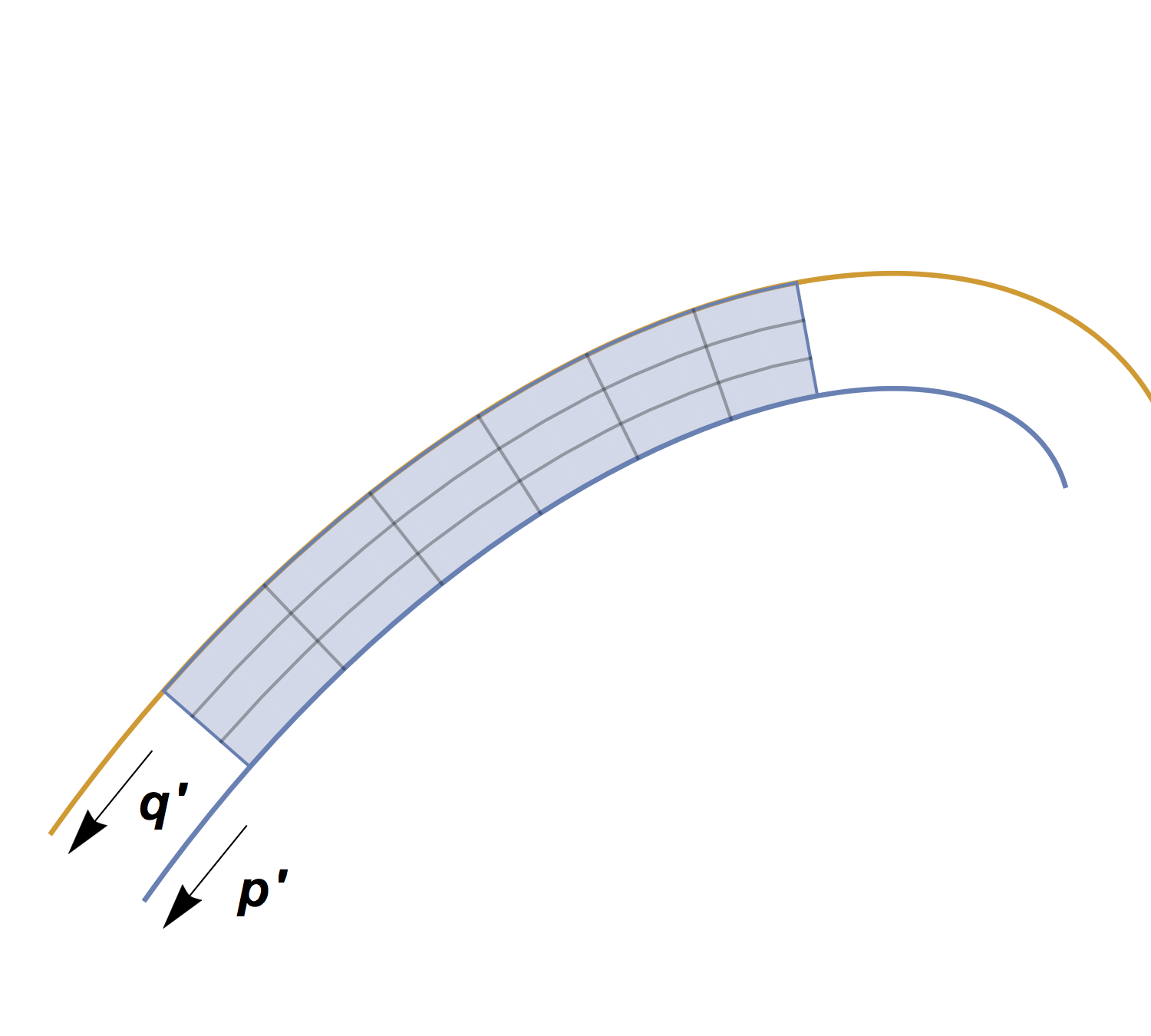
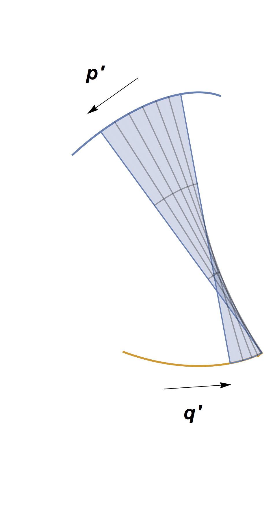
Figure 5: Ribbons and bowties.
A helpful related notion is the best-approximating or osculating circle to \({\bf p}\) and \({\bf q}\). It’s not too hard to see that our rigidity assumption causes the osculating circles to \({\bf p}\) and \({\bf q}\) to be concentric! The osculating center lies along the (shared) normal vector from \({\bf p}\) and \({\bf q}\). Its radius from \({\bf p}\) is \(|\tfrac{1}{\theta'(t)}|\). Thus in the ‘ribbon’ case, \({\bf p}\) and \({\bf q}\) are on the same outward ray from the osculating center. In the ‘bowtie’ case, they are on opposite rays!
So, the condition \(1+d\theta'(t) \geq 0\) says that the curves always remain in ‘ribbon’ form, that they never rotate in ‘bowtie’ form on opposite sides of the osculating center. The latter sort of motion occurs between the former planet Pluto and its moon Charon (they are similar in size, and their collective center of mass lies approximately halfway in between them). More familiarly, it occurs between two spinning contradance partners.
Finally, we note that \(1+d\theta'(t) = 0\) if and only if \({\bf q}'(t) = 0\). In this case \({\bf q}\) will usually have a cusp singularity, instantaneously pausing in place as \({\bf p}\) rotates directly around it.
Ribbons and arclengths
We examine a simple example where the assumptions of Equation \(\eqref{eqn:core_assumption}\) hold, but the arclengths of \({\bf p}\) and \({\bf q}\) do not differ by an integer multiple of \(2\pi d\). Based on the discussion above, this can only occur when \({\bf p}'(t) \cdot {\bf q}'(t) < 0\) for some or all values of \(t\), so the curves must move on opposite sides of the osculating center.
A first case is to consider the spinning contradance partners who, we will assume, have arms of different lengths. Let \(d = a+b\), and let \({\bf p}, {\bf q}\) trace out concentric circles of radii \(a, b\), on opposite sides of a radial center point: \[\begin{align*} {\bf p}(t) &= -a (\cos t, \sin t), \\ {\bf q}(t) &= \ b (\cos t, \sin t). \end{align*}\]Clearly \(||{\bf q}-{\bf p}|| = a+b = d\) for all \(t\), and \({\bf q}' = -\tfrac{b}{a}{\bf p}'\). In this case, the arclengths are \(2\pi a\) and \(2\pi b\), and the difference is \(2\pi(b-a)\), which can be anything from \(0\) to \(2\pi d\).
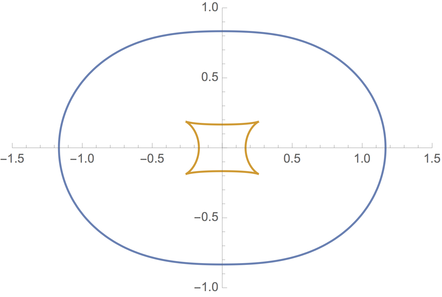
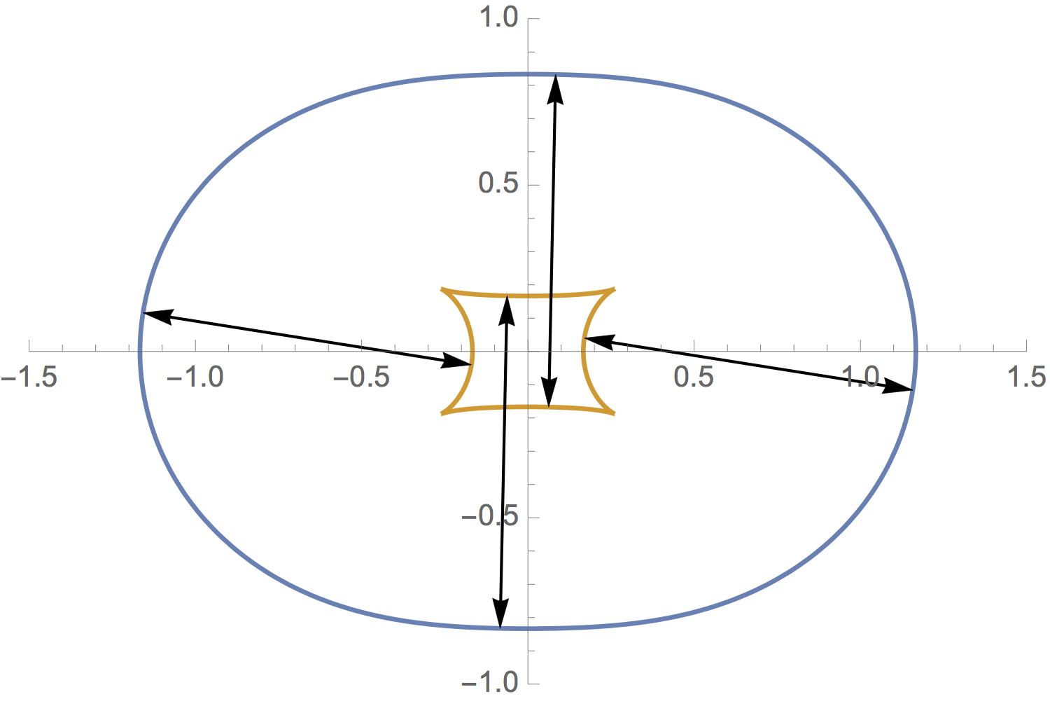
Figure 6: Parallel curves with unusual arclengths! The outer curve has arclength approximately \(6.455\), while the inner curve (at unit distance \(d=1\)) has arclength \(\approx 1.929\). The difference is \(4.526\), which is not a multiple of \(2 \pi\). Note that these curves are traversed in opposite rotational directions: the runner on the outer path goes counterclockwise, and the runner on the inner path goes clockwise. The horizontal parts of the paths are in “ribbon formation” and the vertical parts are in “bowtie formation”.
A more interesting case is the ‘pinched’ curve in Figure 6. In this case the arclength differs by a real number that is not an integer multiple of \(2\pi\), even though \({\bf p}(t)\) and \({\bf q}(t)\) are always unit distance apart. Note that \({\bf p}' \cdot {\bf q}'\) changes sign four times, giving four cusps.