Model

We have a set of \(n\) supply units, which are known in advance, and \(n\) demand units arrive one at a time. Each unit of supply and demand is located in a space \(X\); assume that supply locations are drawn iid from distribution \(F_S\) on \(X\), and demand locations are drawn iid from distribution \(F_D\).

When each demand unit arrives, we must match it to a remaining supply unit. The cost of matching supply at location \(x_s\) to demand at location \(x_d\) is given by a cost function \(c(x_s, x_d)\). Our goal is to minimize total cost.

You can think of this as a stylized version of the problem facing Amazon: it has items (supply) stored in multiple fulfillment centers, and each time a customer orders one, it must immediately decide where to ship the item from.

Algorithm

The algorithm the authors study is simple. Suppose that you have \(k\) units of supply left, and a new demand unit arrives. Sample \(k-1\) future orders from \(F_D\), and determine the lowest-cost way to match your \(k\) supply units to the \(k\) demand units (one real, and \(k-1\) simulated). Match the current demand to whichever supply unit was found to be optimal, and proceed. The authors have named this algorithm SOAR for “Simulate, Optimize, Assign, Repeat.” (I wish I could come up with clever names like that.)

Analysis

The algorithm is super simple – surely it can’t be very good! In fact, the authors show that it is asymptotically optimal in a number of cases. I won’t go into those details, but I will illustrate how nice some of the analysis is.

We will use as a benchmark the solution to the offline optimization problem (where the planner can see all demand locations before deciding how to match). Define \(C_k\) to be the expected per-item cost, when \(k\) random supply units (drawn from \(F_S\)) are matched optimally to \(k\) random demand units (drawn from \(F_D\)).

Theorem. The expected per-item cost of SOAR is \(\frac{1}{n}\sum_{k = 1}^n C_k\).

The key to proving this is the following observation.

Lemma. Given any \(k\) supply units, each supply unit is equally likely to be matched to the subsequent demand unit (before observing the locating of this demand unit).

To see why this is true, imagine that we generate \(k\) random demand units first, and only learn which is the “real” demand after finding the optimal matching for these \(k\) units. Since each supply unit is matched to exactly one demand unit, it follows that each supply unit is equally likely to be matched to the real demand from this period.

This lemma implies that after any number of steps, the remaining supply units are a random subset of the original supply units. From this, it follows fairly immediately that if we start with \(n\) random supply units, then our expected cost from serving the first demand unit is \(C_n\), from serving the second demand unit is \(C_{n-1}\), and so on.

Simulations and Variants

I wrote some R code that uses the igraph library to implement SOAR, as well as the greedy algorithm and the optimal offline algorithm.

library(igraph)

#This function generates k uniformly random points in the 2-D unit square.
#I am assuming F_S = F_D, but this could easily be changed. 
generate_random_points = function(k){
	return(matrix(runif(2*k),ncol=2))
}

#This function calculates euclidean distance
dist = function(x1,x2){ #First element is ID number
	return(sqrt(sum((x1-x2)^2)))
}


#Given n units of supply and demand, this calculates the optimal way to match them
#Return value is an n-dimensional vector, with i^th component indicating supply to which i^th demand was matched
find_opt_matching = function(supply,demand){
	k = length(demand[,1])
	if(length(supply[,1])!=k) print("ERROR: Supply and Demand Unequal Size")
	D = matrix(0,nrow=2*k,ncol=2*k)
	for(i in 1:k) for(j in 1:k){ #sqrt(2)-D ensures all positive entries (because I work in 2-D unit square)
		D[i,j+k] = D[j+k,i] = sqrt(2)-dist(demand[i,],supply[j,]) 
	}
	g = graph_from_adjacency_matrix(D,mode='undirected',weighted=TRUE) 
	V(g)$type = c(rep(TRUE,k),rep(FALSE,k))
	return(max_bipartite_match(g)$matching[1:k]-k) 
}

#M is an n-dimensional vector, with i^th component indicating supply to which i^th demand was matched
find_matching_cost = function(M,supply,demand){
	cost = 0
	for(i in 1:n){ cost = cost+dist(demand[i,],supply[M[i],]) }
	return(cost)
}

#This plots the matching M on a 2-D unit square
plot_matching = function(M,supply,demand,title=''){
	plot(NA,xlim=c(0,1),ylim=c(0,1),xlab='',ylab='',xaxt='n',yaxt='n',main=title)
	n = length(supply[,1])
	points(supply[,1],supply[,2],col='red',pch=21,cex=1.5)
	points(demand[,1],demand[,2],col='blue',pch=as.character(1:n),cex=1.5)
	segments(demand[,1],demand[,2],supply[M,1],supply[M,2])
}

#This runs the modified SOAR algorithm with parameter m on given supply and demand units
#Return value is an n-dimensional vector, with i^th component indicating supply to which i^th demand was matched
SOAR = function(supply,demand,m){
	n = length(supply[,1])
	matched_supply = numeric()
	for(k in n:2){
		remaining_supply = which(!(1:n %in% matched_supply))
		selected_supply = numeric()
		while((length(selected_supply) == 0) || (max(table(selected_supply))<m)){
			simulated_demand = rbind(demand[n-k+1,],generate_random_points(k-1))
			M = find_opt_matching(supply[remaining_supply,],simulated_demand)
			selected_supply = c(selected_supply,remaining_supply[M[1]])
		}
		most_common_supply = as.numeric(names(sort(table(selected_supply),decreasing=TRUE))[1])
		matched_supply = c(matched_supply,	most_common_supply)
	}
	matched_supply = c(matched_supply,which(!(1:n %in% matched_supply))) #Final demand gets matched to whatever supply is left
	return(matched_supply)
}

#An implementation of the greedy algorithm
GREEDY = function(supply,demand){
	n = length(supply[,1])
	matched_supply = numeric()
	for(k in 1:n){
		d = Inf
		for(j in which(!(1:n %in% matched_supply))){
			if(dist(demand[k,],supply[j,]) < d){ d = dist(demand[k,],supply[j,]); best = j; }
		}
		matched_supply = c(matched_supply,best)
	}
	return(matched_supply)
}

Now let’s use this code to actually do something. We’ll start by visualizing a small instance, and how the various alorithms differ.

#Generate a random instance of size 6, compare Optimal, Greedy, and SOAR
set.seed(123456)
n = 6
supply = generate_random_points(n)
demand = generate_random_points(n)

par(mfrow=c(1,3))
#find_matching_cost(find_opt_matching(supply,demand),supply,demand)
plot_matching(find_opt_matching(supply,demand),supply,demand,title='Optimal')

gM = GREEDY(supply,demand)
#find_matching_cost(gM,supply,demand)
plot_matching(gM,supply,demand,title='Greedy')

sM = SOAR(supply,demand,1)
#find_matching_cost(sM,supply,demand)
plot_matching(sM,supply,demand,title='SOAR')

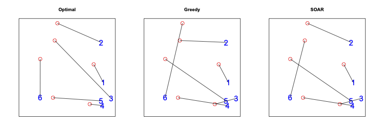
Note that the greedy algorithm matches demand 2 to the closest point, even though it’s pretty clear that the point above it would be a better choice (this point is nearly as close, and unlikely to be close to future demand).

Meanwhile, SOAR matches demand 2 correctly. It’s match for demand 3 is a mistake in hindsight, but was probably the correct decision ex ante: we got relatively unlucky, with three consecutive demand units clustered in the lower right corner, and no demand in the upper left.

One obvious potential downside for SOAR is that you might get an atypical sample of future demand, causing you to make a suboptimal matching choice. The natural solution is to simulate many times, and match the current demand to the supply unit that is chosen most frequently. Specifically, I propose a modified SOAR algorithm where we repeatedly simulate and optimize until one supply unit has been chosen \(m\) times. At this point, we match the current demand to that supply unit. When \(m = 1\), this corresponds to the original SOAR algorithm.

While the analysis of modified SOAR is not as clean as the original, intuitively I would expect its performance to be better. Let’s test that out!

#Generate 100 random instances of size 20, compare different modified SOAR instances
numTrials = 100
n = 20
opt = greedy = soar1 = soar2 = soar3 = soar9 = rep(0,numTrials)
for(t in 1:numTrials){
	supply = generate_random_points(n)
	demand = generate_random_points(n)
	opt[t] = find_matching_cost(find_opt_matching(supply,demand),supply,demand)
	greedy[t] = find_matching_cost(GREEDY(supply,demand),supply,demand)
	soar1[t] = find_matching_cost(SOAR(supply,demand,1),supply,demand)
	soar2[t] = find_matching_cost(SOAR(supply,demand,2),supply,demand)
	soar3[t] = find_matching_cost(SOAR(supply,demand,3),supply,demand)
	soar9[t] = find_matching_cost(SOAR(supply,demand,9),supply,demand)
}
apply(rbind(opt,greedy,soar1,soar2,soar3,soar9),1,mean)

##      opt   greedy    soar1    soar2    soar3    soar9 
## 3.864270 4.837117 5.669992 5.029674 4.907715 4.705098

In this example, we do see that using more simulations seems to get a higher quality (lower cost) solution. Interestingly, the greedy algorithm seems to do pretty well here! At least, better than SOAR with \(m =\) 1, 2, or 3.

Discussion

I love this paper for the simple algorithm and analysis. If you asked me to design an algorithm that was “smarter” than greedy, I could do it, but the resulting algorithm probably would be difficult to explain and analyze, and would depend in a detailed way on the space \(X\) and cost function \(C\).

By contrast, SOAR is easy to implement, and generalizes naturally to many settings. This includes many topological spaces and cost functions, but also totally different online decision problems. For example, I could imagine using this idea for online selection problems (such as prophet inequality problems): simulate future values, and select the present value if it is among the highest.

The SOAR algorithm resembles Thompson sampling, in that once we have revealed the next demand unit, we choose each remaining supply unit with probability equal to the probability that supply unit is ex post optimal (given our previous decisions).

Of course, implementing SOAR requires a good model of future demand, and the guarantees don’t hold if our future demand is drawn from a different distribution than we are using to simulate. However, many algorithms rely on distributional knowledge of future demand, and at least in some cases – such as for Amazon – this doesn’t seem so implausible.