I liked the work, and want to bring it to other’s attention. In this post, I describe some of the main ideas in the paper. An accompanying post presents some new results that I derived after seeing the talk.

1 The Setting

You are presented with a sequence of $n$ values $V_{1}, \dots, V_{n}$ . In period $i$ , you are shown $v_{i}$ , and must make an irrevocable decision to keep or dismiss it. You can keep at most $k$ values, and earn a reward equal to the sum of kept values. You do not initially know ${V_{i}}_{i = 1}^{n}$ , but know that they are drawn independently from distributions $F = {F_{i}}_{i = 1}^{n}$ . We assume that the $F_{i}$ are continuous distributions with finite mean, although all ideas can be extended to the case where the $F_{i}$ are discrete.

Although one could solve for the optimal policy using dynamic programming, we will instead focus on a class of much simpler policies.

Static Threshold Policies. Set a static threshold $t$ . Keep item $i$ if and only if $V_{i} > t$ and fewer than $k$ items have been kept so far. Let $S T_{k}^{t} (F)$ denote the expected performance of this policy.

We will benchmark these policies against a “prophet” who knows the values $V_{i}$ in advance, and keeps the $k$ highest.

Omniscient Benchmark. Let $O M N_{k} (F)$ denote the expected sum of the $k$ highest values.

We wish to know, if we choose the threshold $t$ well, how much worse can a static threshold policy be than the omniscient solution? In other words, we want to compute $inf_{F} sup_{t} \frac{S T_{k}^{t} (F)}{O M N_{k} (F)} .$

Computing this value is hard, so this paper gives a lower bound by (i) proposing an elegant way to choose $t$ , and (ii) analyzing the resulting performance.

2 What Was Already Known?

The most studied case is $k = 1$ . In that case, it is well-known that a suitable static threshold guarantees half of the omniscient value. (This is actually a pretty amazing fact, when you think about it.) No better guarantee is possible, as the following simple example shows that even the optimal policy guarantees only half of the omniscient value. Let $V_{1}$ be deterministically equal to 1, and let $V_{2}$ be $1 / ϵ$ with probability $ϵ$ , and $0$ otherwise. Any optimal policy obtains expected reward of $1$ , whereas the omniscient policy obtains expected reward of $2 - ϵ$ .

There are several ways to choose the threshold $t$ to guarantee $1 / 2$ of omniscient. One especially elegant method from Samuel-Cahn (1984) is the “median strategy”: take $t$ to be the median of the distribution of the maximum of the $V_{i}$ . Another approach is the “mean strategy” of Kleinberg and Weinberg (2012): take $t$ to be half of the mean of the distribution of the maximum of the $V_{i}$ .

The latter approach generalizes to the case $k > 1$ , producing an identical guarantee of $1 / 2$ . However, this guarantee is far from optimal. When $k$ is large, the law of large numbers kicks in, and you can do pretty well by choosing a threshold $t$ such that the expected number of items with value above $t$ is just a bit below $k$ . Hajiaghayi, Kleinberg and Sandholm (2007) show that static threshold policies can achieve a fraction of $O M N$ that is $1 - O (\sqrt{\log (k) / k})$ . Note in particular that this guarantee goes to $1$ as $k \to \infty$ . However, the constants established in that work are such that for $k \leq 20$ , the best known guarantee is $1 / 2$ .

3 Their Algorithm and Results

The goal of the paper is to generalize the median strategy to arbitrary $k > 1$ .

3.1 Key Step #1: Balancing Two Risks

When setting

t

, we face a tradeoff. Set

t

too high, and we might not keep very many items. Set

t

too low, and we might might take

k

items early, and miss out on a valuable item later. The crux of the algorithm will be to find a way to balance these concerns. Define

\begin{aligned} (1) & D_{t} (V) & = \sum_{i = 1}^{n} 1 (V_{i} > t) \\ (2) & δ_{k} (t, F) & = P_{V \sim F} (D_{t} (V) < k) \\ (3) & μ_{k} (t, F) & = \frac{1}{k} E_{V \sim F} [min (D_{t} (V), k)] \end{aligned}

That is, $D_{t} (V)$ is the “demand” at $t$ (number of values above $t$ ), $δ_{k}$ gives the probability of keeping fewer than $k$ items when using threshold $t$ , and $μ_{k}$ is our expected “fill rate” (the expected number of items that we keep, divided by $k$ ). The following result relates the performance of $S T_{k}^{t}$ to $δ_{k}$ and $μ_{k}$ .

Proposition 3.1 For all

F

k

t

, we have

\frac{S T_{k}^{t} (F)}{O M N_{k} (F)} \geq min (δ_{k} (t, F), μ_{k} (t, F)) .

The key idea is that when we consider any value $V_{i}$ , the probability that we have not yet kept $k$ items (and could therefore choose $V_{i}$ if we wish) is at least $δ_{k}$ . Meanwhile, if $μ_{k}$ is high, then we don’t lose much due to keeping too few items.

An Algorithm For Choosing $t$ . Proposition 3.1 immediately implies the following. $inf_{F} sup_{t} \frac{S T_{k}^{t} (F)}{O M N_{k} (F)} \geq inf_{F} sup_{t} min (δ_{k} (t, F), μ_{k} (t, F)) .$

This suggests an algorithm for choosing $t$ : since $δ_{k}$ is increasing in $t$ , and $μ_{k}$ is decreasing in $t$ , the supremum is obtained at a threshold $t$ such that $δ_{k} (t, F) = μ_{k} (t, F)$ . When $k = 1$ , we have $μ_{1} (t, F) = 1 - δ_{1} (t, F)$ for all $t$ and $F$ . This implies that at their crossing point, both are equal to $1 / 2$ . In other words, we set a threshold $t$ such that our probability of keeping any item is $1 / 2$ : this is the median algorithm of Samuel-Cahn (1984)!

Notes on the Proof. The proof establishes a lower bound on

S T_{k}^{t} (F)

, expressed in terms of the following function:¹

\begin{matrix} (4) & U (t, F) = E_{V \sim F} [\sum_{i = 1}^{n} max (V_{i} - t, 0)] = \sum_{i = 1}^{n} \int_{t}^{\infty} (1 - F_{i} (x)) d x . \end{matrix}

The second inequality above uses my one of my favorite facts: for a non-negative random variable

X

E [X] = \int_{0}^{\infty} P (X > x) d x .

Lemma 3.1 For all

t, k, F

, we have

S T_{k}^{t} (F) \geq μ_{k} (t, F) \cdot k \cdot t + δ_{k} (t, F) \cdot U (t, F)

It also establishes an upper bound on OMN. Define

\begin{matrix} (5) & B_{k} (t, F) = k \cdot t + U (t, F) . \end{matrix}

Lemma 3.2 For all

t, k, F

, we have

O M N_{k} (F) \leq B_{k} (t, F) .

Jointly, Lemmas 3.1 and 3.2 imply Proposition 3.1. In fact, the resulting guarantee holds even against the benchmark of an LP relaxation of OMN, which is permitted to keep at most $k$ values in expectation, rather than for every realization. This relaxation sets a threshold $t_{k}^{L P} (F)$ such that the expected demand is equal to $k$ , and then accepts all such items. Its expected payout is $L P_{k} (F) = E_{V \sim F} [\sum_{i = 1}^{n} V_{i} 1 (V_{i} > t_{k}^{L P} (F))] = min_{t} B_{k} (t, F) .$

3.2 Key Step #2: Determining the Worst Case

We now need to find a worst case choice of the distributions $F$ . One key advantage of this analysis is that the functions $δ_{k}$ and $μ_{k}$ depend only on the distribution of $D_{t} (V)$ , which is a sum of independent Bernoulli random variables. Therefore, instead of optimizing over the space of all distributions, it is enough to optimize over the success probabilities (referred to as “biases” in the paper) $b_{i} = (1 - F_{i} (t))$ .

The most involved step in their analysis is to show that the worst case is when the biases are equal, and $D_{t}$ follows a binomial distribution. We let $X_{n, p}$ denote a binomial random variable with $n$ trials and success probability $p$ .

Proposition 3.2 For all

n, k

inf_{F} sup_{t} min (δ_{k} (t, F), μ_{k} (t, F)) \geq sup_{p \in [0, 1]} min (\frac{1}{k} E [min (X_{n, p}, k)], P (X_{n, p} < k)) = γ_{k, n} .

We can use the following code to compute the values $γ_{k, n}$ .

delta_binom = function(n,k,p){
  return(pbinom(k-1,n,p))
}
mu_binom = function(n,k,p){
  prob = dbinom(0:(k-1),n,p)
  prob = c(prob,1-sum(prob))
  return(sum(prob*c(0:k))/k)
}
guarantee_at_p = function(n,k){
  return(Vectorize(function(p){return(min(delta_binom(n,k,p),mu_binom(n,k,p)))}))
}
guarantee_finite = Vectorize(function(n,k){
  return(optimize(guarantee_at_p(n,k),interval=c(0,1),maximum=TRUE)$objective)
})
kVals = c(2:4)
colors = rainbow(length(kVals))
nMax = 10 
plot(NULL,xlim=c(2,nMax),ylim=c(0.5,0.75),las=1,xlab='n',ylab='',main='Performance Guarantee')
for(i in 1:length(kVals)){
  lines(c(kVals[i]:nMax),guarantee_finite(c(kVals[i]:nMax),kVals[i]),col=colors[i])
}
legend(2,.58,col=colors,lty=rep('solid',length(kVals)),legend = kVals)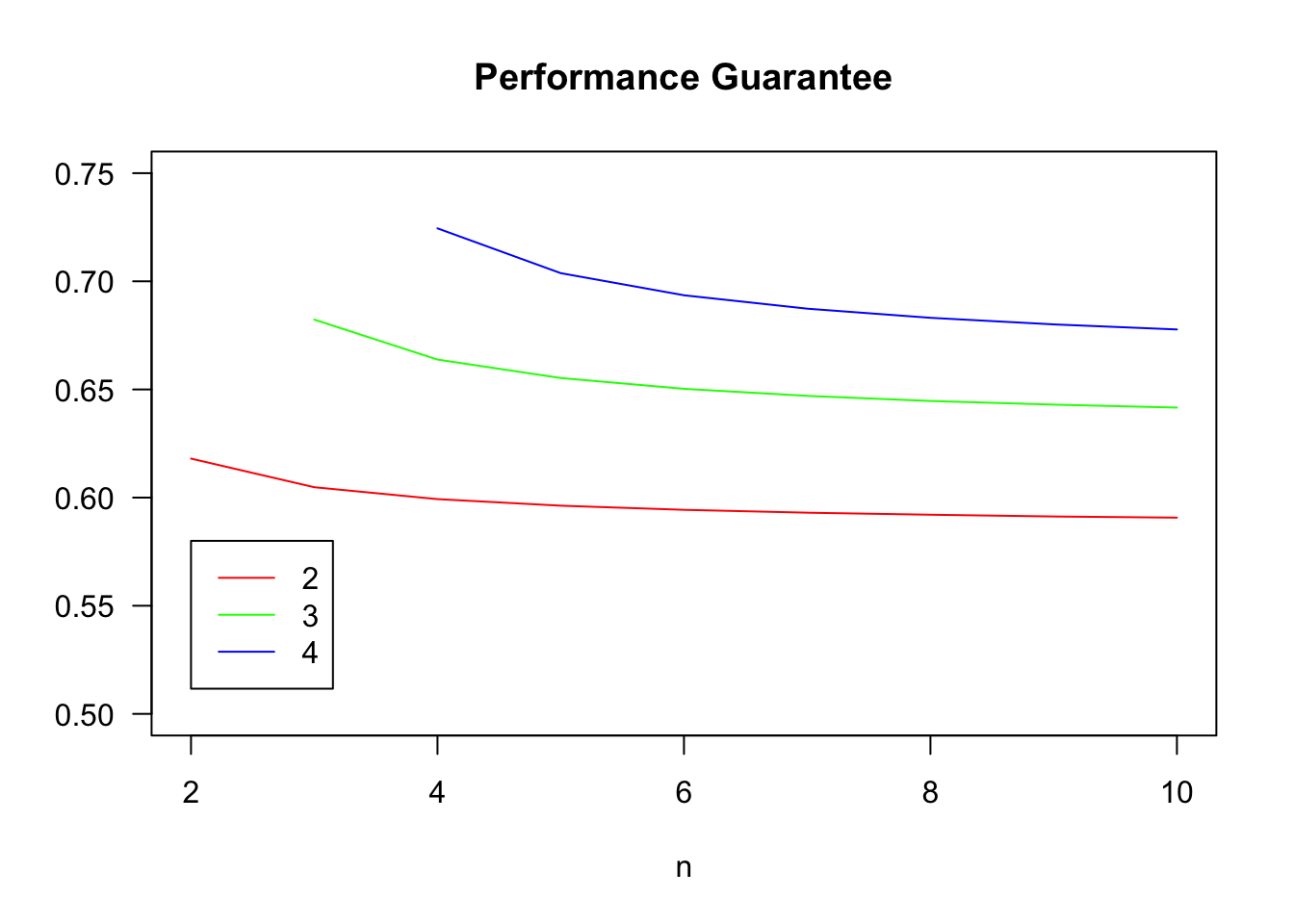

The guarantee $γ_{k, n}$ is increasing in $k$ and decreasing in $n$ , but depends much more on $k$ than $n$ . If we take $n \to \infty$ , the binomial distribution becomes a Poisson, and we obtain bounds that hold for all $n$ .

delta_pois = function(lambda,k){return(ppois(k-1,lambda))}
mu_pois = function(lambda,k){
  prob = dpois(0:(k-1),lambda)
  prob = c(prob,1-sum(prob))
  return(sum(prob*c(0:k))/k)
}
guarantee_at_lambda = function(k){
  return(Vectorize(function(lambda){
    return(min(delta_pois(lambda,k),mu_pois(lambda,k)))
  }))
}
guarantee_pois = Vectorize(function(k){
  return(optimize(guarantee_at_lambda(k),interval=c(0,k),maximum=TRUE)$objective)
})
kVals = c(1:10)
round(guarantee_pois(kVals),3)

##  [1] 0.500 0.586 0.631 0.660 0.682 0.699 0.713 0.724 0.734 0.742

For $k = 1$ , we recover the guarantee of $1 / 2$ , but this paper provides the first guarantee above $1 / 2$ for $k = 2$ . The guarantee converges to $1$ (at an optimal rate) as $k \to \infty$ .

4 Closing Thoughts

What do I like about this paper?

It asks a clean question: I appreciate the simplicity of static threshold policies.
It offers a simple policy. Although the optimal threshold depends on the order in which the $V_{i}$ are presented, the authors’ proposed choice of $t$ does not.
The analysis is elegant:
- The first step offers clear intuition about balancing the risks of setting the threshold too high and too low.
- The second step leverages the fact that their bound depends only on the values $1 - F_{i} (t_{i})$ , rather than the full distributions $F_{i}$ .
The final result is a tight analysis of the performance of their policy.
The paper is written exceptionally clearly throughout, and is a joy to read.

The authors seem to have found the “right” generalization of the Samuel-Cahn median strategy, which is not at all obvious: Kleinberg and Weinberg (2012) write “it is hard to surpass the elegance of Samuel-Cahn’s proof”, but argue that the advantage of their approach is that “it generalizes to arbitrary matroids.” Meanwhile, these lecture notes call the median strategy “beautiful,” but “somewhat mysterious, and difficult to generalize.”

One special case of interest is when the $V_{i}$ are iid. Although this seems like an easier setting, simple examples show that their algorithm’s performance may match the lower bound of $γ_{k, n}$ even with iid values. In this follow-up post, I explore a simple algorithm that improves upon this guarantee.

The authors use an extended analogy linking this setting to one in which an auctioneer has $k$ copies of an item and wishes to allocate them to the buyers with the highest values. The quantity $U$ can thus be interpreted as the total buyer surplus if each buyer allowed to purchase for price $t$ .↩

nikhil devanur

0 points

5 years ago

Meanwhile, these lecture notes call the median strategy “beautiful,” but “somewhat mysterious, and difficult to generalize.” This is continued as, "Indeed, suppose we are allowed to choose up to k variables to maximize the sum of their realizations? The above proof seems difficult to generalize, "

Static Pricing for Multi-Unit Prophet Inequalities

Nick Arnosti

2020/09/25

1 The Setting

2 What Was Already Known?

3 Their Algorithm and Results

3.1 Key Step #1: Balancing Two Risks

3.2 Key Step #2: Determining the Worst Case

4 Closing Thoughts