1 Setting the Stage

The original paper considers a setting where we are presented with a sequence of values. Each value \(V_i\) is drawn from a known distribution \(F_i\). We are allowed to "keep" at most \(k\) values, and wish to maximize the sum of kept values. We will use a simple static threshold algorithm, which keeps the first \(k\) values above some fixed threshold \(t\). We wish to benchmark the performance of this algorithm against that of an omniscient benchmark that always keeps the \(k\) highest values. The original paper provides an algorithm for choosing \(t\), and a tight analysis of its performance. The following code computes its competitive ratio, as a function of \(k\) (see my preceding post for more explanation):

delta_pois = function(lambda,k){return(ppois(k-1,lambda))}
mu_pois = function(lambda,k){
  prob = dpois(0:(k-1),lambda)
  prob = c(prob,1-sum(prob))
  return(sum(prob*c(0:k))/k)
}
guarantee_at_lambda = function(k){
  return(Vectorize(function(lambda){
    return(min(delta_pois(lambda,k),mu_pois(lambda,k)))
  }))
}
guarantee_pois = Vectorize(function(k){
  return(optimize(guarantee_at_lambda(k),interval=c(0,k),maximum=TRUE)$objective)
})
round(guarantee_pois(c(1:10)),3)

##  [1] 0.500 0.586 0.631 0.660 0.682 0.699 0.713 0.724 0.734 0.742

This post will consider a simpler setting where the \(F_i\) are iid. This should be an easier problem, so we might hope to get a better guarantee. However, the guarantee of their algorithm does not improve! Their algorithm sets a threshold such that the expected number of items kept divided by \(k\) is equal to the guarantee computed above. Therefore, if all values are "nearly deterministic" (i.e. \(U[1-\epsilon,1+\epsiloin]\)), its performance will be approximately equal to their guarantee.

In this post, I show the following:

1. We can get a better guarantee by using a threshold such that the expected "demand" (number of values exceeding the threshold) is equal to \(k\).
2. This algorithm provides the best guarantee among the natural class of "expected demand" policies.

2 The LP Approximation Policy

Their policy's performance is hurt by the fact that it sets too high of a threshold (keeps too few items). To get a better guarantee, we must set a lower threshold, but how much lower?

In the previous post we defined the "demand" at \(t\) to be the number of values exceeding \(t\): \[D_t(V) = \sum_{i = 1}^n {\bf 1}(V_i > t).\] We'll start by considering a natural policy: use the threshold \(t^{LP}\) such that the expected demand is equal to \(k\). We can analyze its performance as follows.

For any threshold \(t\), we have \(D_t \sim Binom(n,1-F(t)).\) We keep \(\min(D_t(V),k)\) values, each with expected value \(\mathbb{E}_{V \sim F}[V \vert V > t]\). Meanwhile, the LP relaxation discussed in my previous post gives an upper bound of \(k \cdot \mathbb{E}_{V \sim F}[V \vert V > t^{LP}]\). Combining these, we get the following performance guarantee: \[\frac{ST_k^{t^{LP}}(F)}{LP_k(F)} = \frac{\mathbb{E}[\min(D_{t^{LP}}(V),k)] \cdot\mathbb{E}_{V \sim F}[V \vert V > t^{LP}]}{k\cdot \mathbb{E}_{V \sim F}[V \vert V > t^{LP}]}\hspace{.3 in} = \frac{\mathbb{E}[\min(Binom(n,k/n),k)]}{k}. \]

For any \(k\), this expression falls as \(n\) grows. In the limit as \(n \rightarrow \infty\), the Binomial becomes a Poisson, yielding the following bounds.

mu_binom = function(n,k,p){
  prob = dbinom(0:(k-1),n,p)
  prob = c(prob,1-sum(prob))
  return(sum(prob*c(0:k))/k)
}
iid_guarantee = Vectorize(function(n,k){return(mu_binom(n,k,k/n))}) #For finite k, n
iid_guarantee_pois = Vectorize(function(k){return(mu_pois(k,k))}) #Limit as n -> \infty
round(iid_guarantee_pois(c(1:10)),3)

##  [1] 0.632 0.729 0.776 0.805 0.825 0.839 0.851 0.860 0.868 0.875

Let's compare these to the bounds obtained for the general case. For \(k = 1\), the bound improves from \(1/2\) to \(1 - 1/e\). Even for very large \(k\), there remains a sizeable gap. For example, with \(k = 100\), the general bound is \(0.88\), and the iid bound is \(0.96\).

kVals = c(1:100)
colors = c('blue','red')
plot(NULL,xlim=c(min(kVals),max(kVals)),ylim=c(0.4,1),las=1,xlab='k',ylab='',main='Performance Guarantee',cex.axis=2,cex.lab=2,cex.main=2)
lines(kVals,iid_guarantee_pois(kVals),col=colors[1],lwd=2)
lines(kVals,guarantee_pois(kVals),col=colors[2],lwd=2)
legend(.62*max(kVals),.65,col=colors,lty=c('solid','solid'),lwd=2,legend = c('IID','General'),cex=1.5)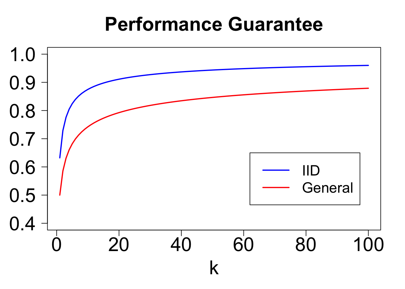

3 Expected Demand Policies

The preceding analysis establishes a performance guarantee for the threshold \(t^{LP}\). But is this threshold optimal? For most \(F\), it is not. However, in we will show that this selection provides the best worst-case guarantee among the following subset of static threshold policies.

Expected Demand Policy. Given \(\alpha > 0\), choose a threshold \(t\) such that expected demand \(n(1 - F(t))\) is equal to \(\alpha \cdot k\).

We denote the performance of this policy on distribution \(F\) by \(ED_k^{\alpha}({\bf F})\).

One way to think of expected demand policies is that they specify the threshold as a fixed quantile of the distribution \(F\). If the quantile can depend on \(n, k,\) and \(F\), then the set of expected demand policies coincides with the set of static threshold policies. However, we will ask the question, can we choose an \(\alpha\) that works well simultaneously for all \(n,k,F\)? To start, we fix \(n\) and \(k\), and solve the following problem: \[\sup \limits_\alpha \inf \limits_{F} \frac{ED_k^\alpha(F)}{LP_k(F)}.\]

Our preceding analysis was for \(\alpha = 1\). It turns out that no other choice of \(\alpha\) offers a better guarantee.

The intuition is as follows. If \(\alpha < 1\), the guarantee will be poor if values are nearly deterministic (we will keep too few values). If \(\alpha > 1\), the guarantee will be poor if the distribution puts a tiny amount of weight on an immense value (we will too often reach our quota and miss out on a very high value).

We can formalize this as follows. Let \(B_{n,p}\) denote a binomial with parameters \(n\) and \(p\). For any \(\alpha < 1\), let \(F\) be uniform on \([1-\epsilon,1+\epsilon]\). As \(\epsilon \rightarrow 0\), our competitive ratio converges to the expected number of values we keep, divided by \(k\): \[\frac{ED_k^\alpha(F)}{OPT_k(F)} \rightarrow \frac{\mathbb{E}[\min(B_{n,\alpha\cdot k/n},k)]}{k}\]

For any \(\alpha > 1\), let \(F\) be such that \(v_i\) is \(1/\epsilon^2\) with probability \(\epsilon\), and otherwise is uniform on \([0,1]\). If \(\epsilon\) is small, all that really matters is how often we keep large values. The optimal policy will save spots for a large value, whereas the \(ED_k^\alpha\) policy will sometimes run out of room. In particular, as \(\epsilon \rightarrow 0\), the competitive ratio will converge to \[\frac{ED_k^\alpha(F)}{OPT_k(F)}= \frac{\mathbb{E}[\min(B_{n,\alpha\cdot k/n},k)]}{\alpha k}.\]

With a little work, we can show that for any \(\alpha\), one of these families of distributions is the worst case, so the competitive ratio for the expected demand policy with parameter \(\alpha\) is \[\frac{\mathbb{E}[\min(B_{n,\alpha \cdot k/n},k)]}{\max(\alpha,1)\cdot k}.\]

As \(n\) grows, this bound falls, and the binomial converges to a Poisson. We can therefore plot the worst-case performance of an expected demand policy as a function of \(\alpha\) and \(k\). For all \(k\), the optimal choice of \(\alpha\) is one, and the guarantee offered by this policy improves with \(k\).

iid_guarantee_alpha = Vectorize(function(alpha,k){return(mu_pois(alpha*k,k)/max(alpha,1))})
alphaMax = 3
plot(NULL,las=1,xlim=c(0,alphaMax),ylim=c(0,1),xlab=expression(alpha),ylab='',main='Performance of Expected Demand Policy',cex.lab=2,cex.axis=2,cex.main=2)
k = c(1,2,5,20)
colors = c('black','red','blue','green')
for(i in 1:length(k)){
  plot(Vectorize(function(x){return(iid_guarantee_alpha(x,k[i]))}),xlim=c(0,alphaMax),col=colors[i],lwd=2,add=TRUE)
}
legend(2.15,1,col=colors,lty=rep('solid',length(k)),lwd=2,legend=c('k=1','k=2','k=5','k=20'),cex=1.5)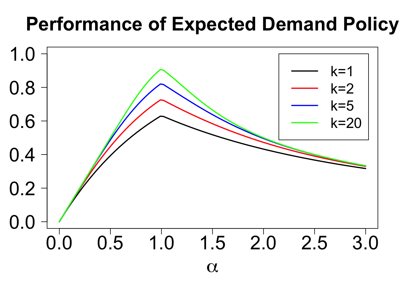

4 Closing Remarks

This post has showed when values are iid, a very simple policy achieves a significant improvement over the guarantees that are known for the non-iid case. While this policy offers the best guarantee of any "expected demand" policy, I don't know whether the resulting bounds are tight for the class of static threshold policies. It would be interesting to see if there is a distribution \(F\) for which no choice of threshold offers a better guarantee.

Another interesting direction of study is an intermediate case, where the values are drawn from different distributions, but presented in a random (rather than fixed) order. This has been dubbed the "Prophet Secretary" problem by some recent papers ("Prophet" coming from the fact that the distributions are known, and "Secretary" from the well-known secretary problem in which adversarially chosen values are presented in random order). Stay tuned for new results in this case!